Model Migration

This chapter mainly gives a brief introduction to the dataset, model, and training and inference processes necessary for model migration scenarios to be built on MindSpore. It also shows the differences between MindSpore and PyTorch in terms of dataset packing, model building, and training process code.

Model Analysis

Before conducting a formal code migration, you need to do some simple analysis of the code that will be migrated to determine which code can be reused directly and which code must be migrated to MindSpore.

In general, only hardware-related code sections have to be migrated to MindSpore, for example:

Related to model input, including model parameter loading, dataset packaging, etc;
Code for model construction and execution;
Related to model output, including model parameter saving, etc.

Third parties that compute on the CPU like Numpy, OpenCV, as well as Python operations like Configuration and Tokenizer that don't require elevation or GPU processing, can directly reuse the original code.

Dataset Packing

MindSpore provides a variety of typical open source datasets for parsing and reading, such as MNIST, CIFAR-10, CLUE, LJSpeech, etc. For details, please refer to mindspore.dataset.

Customized Data Loading GeneratorDataset

In migration scenarios, the most common way to load data is GeneratorDataset, which can be directly docked to the MindSpore model for training and inference by simply packing the Python iterator.

import numpy as np
from mindspore import dataset as ds

num_parallel_workers = 2  # Number of multithreads/processes
world_size = 1            # For parallel scenario, communication group_size
rank = 0                  # For parallel scenario, communication rank_id

class MyDataset:
    def __init__(self):
        self.data = np.random.sample((5, 2))
        self.label = np.random.sample((5, 1))

    def __getitem__(self, index):
        return self.data[index], self.label[index]

    def __len__(self):
        return len(self.data)

dataset = ds.GeneratorDataset(source=MyDataset(), column_names=["data", "label"],
                              num_parallel_workers=num_parallel_workers, shuffle=True,
                              num_shards=1, shard_id=0)
train_dataset = dataset.batch(batch_size=2, drop_remainder=True, num_parallel_workers=num_parallel_workers)

A typical dataset is constructed as above: to construct a Python class, there must be __getitem__ and __len___ methods, which represent the size of the data taken at each step of the iteration and the size of the entire dataset traversed once, respectively, where index represents the index of the data taken at each step, and which is incremented sequentially when shuffle=False, and randomly disrupted when shuffle=True.

GeneratorDataset needs to contain at least:

source: a Python iterator;
column_names: the name of each output of the iterator__getitem__ method.

For more use methods, refer to GeneratorDataset.

dataset.batch takes consecutive batch_size entries in the dataset and combines them into a single batch, which needs to contain at least:

batch_size: Specifies the data entries contained in each batch of data.

For more use methods, refer to Dataset.batch.

Differences with PyTorch Dataset Construction

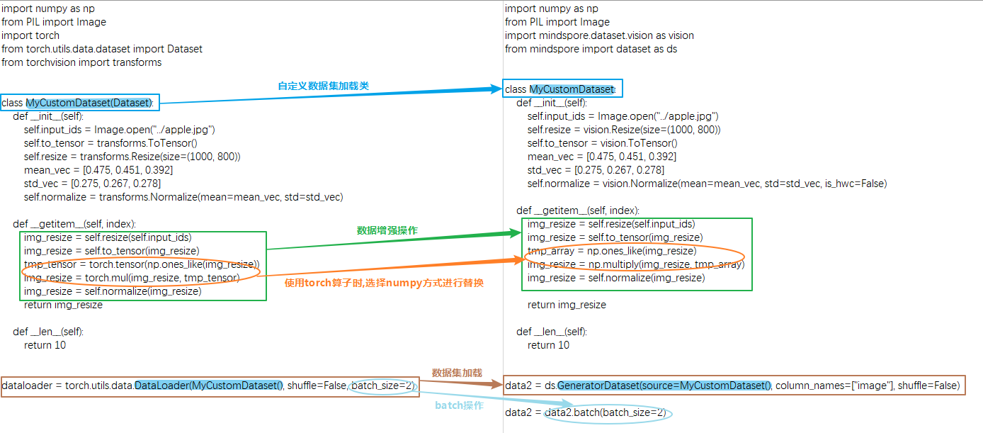
The main differences between MindSpore's GeneratorDataset and PyTorch's DataLoader are:

column_names must be passed in MindSpore's GeneratorDataset;
PyTorch's data augmentation inputs are of type Tensor, MindSpore's data augmentation inputs are of type numpy, and data processing cannot be done with MindSpore's mint, oops, and nn operators;
PyTorch's batch operation is a property of the DataLoader, MindSpore's batch operation is a separate method.

For more details, refer to Differences with torch.utils.data.DataLoader.

Model Construction

Fundamental Building Block of Network Cell

MindSpore's network construction mainly uses Cell for graph construction. Users need to define a class to inherit Cell as the base class, declare the APIs and sub-modules to be used in init, and carry out calculations in construct:

PyTorch

MindSpore

import torch

class Network(torch.nn.Module):
    def __init__(self, forward_net):
        super(Network, self).__init__()
        self.net = forward_net

    def forward(self, x):
        y = self.net(x)
        return torch.nn.functional.relu(y)

inner_net = torch.nn.Conv2d(120, 240, kernel_size=4, bias=False)
net = Network(inner_net)
for i in net.parameters():
    print(i)

from mindspore import mint, nn

class Network(nn.Cell):
    def __init__(self, forward_net):
        super(Network, self).__init__()
        self.net = forward_net

    def construct(self, x):
        y = self.net(x)
        return mint.nn.functional.relu(y)

inner_net = mint.nn.Conv2d(120, 240, kernel_size=4, bias=False)
net = Network(inner_net)
for i in net.get_parameters():
    print(i)

MindSpore and PyTorch build models in pretty much the same way, and the differences in the use of operators can be found in the API Differences document.

Model Saving and Loading

PyTorch provides state_dict() for parameter state viewing and saving, and load_state_dict for model parameter loading.

MindSpore can use save_checkpoint and load_checkpoint.

PyTorch

MindSpore

# Use torch.save() to save the obtained state_dict to a pkl file
torch.save(pt_model.state_dict(), save_path)

# Load the saved state_dict using torch.load().
# Then use load_state_dict to load the obtained state_dict into the model
state_dict = torch.load(save_path)
pt_model.load_state_dict(state_dict)

# Model weight saving
ms.save_checkpoint(ms_model, save_path)

# Load the saved ckpt file using ms.load_checkpoint().
# Then load the obtained param_dict into the model using load_state_dict
param_dict = ms.load_checkpoint(save_path)
ms_model.load_state_dict(param_dict)

Optimizer

Comparison of similarities and differences between optimizers supported by both PyTorch and MindSpore, see API mapping table.

Implementation and Usage Differences of Optimizers

When PyTorch executes the optimizer in a single step, it usually needs to manually execute the zero_grad() method to set the historical gradient to 0, then use loss.backward() to compute the gradient of the current training step, and finally call the step() method of the optimizer to implement the update of the network weights;

When using the optimizer in MindSpore, simply compute the gradients directly and then use optimizer(grads) to perform the update of the network weights.

If the learning rate needs to be dynamically adjusted during training, PyTorch provides the LRScheduler class for learning rate management. When using dynamic learning rates, pass the optimizer instance into the LRScheduler subclass and perform the learning rate modification by calling scheduler.step() in a loop and synchronizing the modification to the optimizer.

MindSpore provides both Cell and list methods for dynamically modifying the learning rate. When used, the corresponding dynamic learning rate object is passed directly into the optimizer, and the update of the learning rate is executed automatically in the optimizer, please refer to Dynamic Learning Rate.

PyTorch

MindSpore

optimizer = optim.SGD(model.parameters(), lr=0.01, momentum=0.9)
scheduler = ExponentialLR(optimizer, gamma=0.9)

optimizer.zero_grad()
output = model(input)
loss = loss_fn(output, target)
loss.backward()
optimizer.step()
scheduler.step()

import mindspore
from mindspore import nn

lr = nn.exponential_decay_lr(0.01, decay_rate, total_step, step_per_epoch, decay_epoch)

optimizer = nn.SGD(model.trainable_params(), learning_rate=lr, momentum=0.9)
grad_fn = mindspore.value_and_grad(forward_fn, None, optimizer.parameters, has_aux=True)
(loss, _), grads = grad_fn(data, label)
# Automatically perform learning rate updates in the optimizer
optimizer(grads)

Automatic Differentiation

Both MindSpore and PyTorch provide auto-differentiation, allowing us to define a forward network and then implement automatic backpropagation as well as gradient updating with a simple interface call. However, it should be noted that MindSpore and PyTorch have different logics for building backward graphs, and this difference can also lead to differences in API design.

Automatic Differentiation in PyTorch

Automatic Differentiation in MindSpore

# torch.autograd:
# The backward is cumulative and the optimizer needs to be cleared after the update.

import torch.nn as nn
import torch.optim as optim

# Instantiating Models and Optimizers
model = PT_Model()
optimizer = optim.SGD(model.parameters(), lr=0.01)

# Define the loss function: mean square error (MSE)
loss_fn = nn.MSELoss()

# Forward propagation: calculating model output
y_pred = model(x)

# Calculating losses: calculate losses by comparing predicted values with true labels
loss = loss_fn(y_pred, y_true)

# Backpropagation: calculating the gradient
loss.backward()
# Optimizer Update
optimizer.step()

# ms.grad:
# Use the grad interface to input a forward graph and output a backward graph
import mindspore as ms
from mindspore import nn

# Instantiating Models and Optimizers
model = MS_Model()
optimizer = nn.SGD(model.trainable_params(), learning_rate=0.01)

# Define the loss function: mean square error (MSE)
loss_fn = nn.MSELoss()

def forward_fn(x, y_true):
    # Forward propagation: computing model output
    y_pred = model(x)
    # Computing losses: calculate losses by comparing predicted values with true labels
    loss = loss_fn(y_pred, y_true)
    return loss, y_pred

# Calculate the loss and gradient
grad_fn = ms.value_and_grad(forward_fn, None, optimizer.parameters, has_aux=True)
(loss, _), grads = grad_fn(x, y_true)
# Optimizer Update
optimizer(grads)

Model Training and Inference

The following is an example of Trainer in MindSpore, which contains training and training-time inference. The training part mainly contains combining modules such as dataset, model, and optimizer for training; the inference part mainly contains evaluating the metrics acquisition, saving the optimal model parameters, and so on.

import mindspore as ms
from mindspore import nn
from mindspore.amp import StaticLossScaler, all_finite
from mindspore.communication import init, get_group_size

class Trainer:
    """A training example with two losses"""
    def __init__(self, net, loss1, loss2, optimizer, train_dataset, loss_scale=1.0, eval_dataset=None, metric=None):
        self.net = net
        self.loss1 = loss1
        self.loss2 = loss2
        self.opt = optimizer
        self.train_dataset = train_dataset
        self.train_data_size = self.train_dataset.get_dataset_size()    # Obtain the number of batch in the training set
        self.weights = self.opt.parameters
        # Note that the first argument to value_and_grad needs to be the graph for which the gradient derivation needs to be done, typically containing the network and the loss. Here it can be a function or a Cell
        self.value_and_grad = ms.value_and_grad(self.forward_fn, None, weights=self.weights, has_aux=True)

        # For distributed scenario
        self.grad_reducer = self.get_grad_reducer()
        self.loss_scale = StaticLossScaler(loss_scale)
        self.run_eval = eval_dataset is not None
        if self.run_eval:
            self.eval_dataset = eval_dataset
            self.metric = metric
            self.best_acc = 0

    def get_grad_reducer(self):
        grad_reducer = nn.Identity()
        # Determine whether the scenario is distributed. For distributed scenario settings, refer to the above general runtime environment settings
        group_size = get_group_size()
        reducer_flag = (group_size != 1)
        if reducer_flag:
            grad_reducer = nn.DistributedGradReducer(self.weights)
        return grad_reducer

    def forward_fn(self, inputs, labels):
        """Forward network construction, note that the first output must be the last one to require a gradient"""
        logits = self.net(inputs)
        loss1 = self.loss1(logits, labels)
        loss2 = self.loss2(logits, labels)
        loss = loss1 + loss2
        loss = self.loss_scale.scale(loss)
        return loss, loss1, loss2

    @ms.jit    # jit acceleration, need to meet the requirements of graph pattern builds, otherwise it will report an error
    def train_single(self, inputs, labels):
        (loss, loss1, loss2), grads = self.value_and_grad(inputs, labels)
        loss = self.loss_scale.unscale(loss)
        grads = self.loss_scale.unscale(grads)
        grads = self.grad_reducer(grads)
        self.opt(grads)
        return loss, loss1, loss2

    def train(self, epochs):
        train_dataset = self.train_dataset.create_dict_iterator(num_epochs=epochs)
        self.net.set_train(True)
        for epoch in range(epochs):
            # Training an epoch
            for batch, data in enumerate(train_dataset):
                loss, loss1, loss2 = self.train_single(data["image"], data["label"])
                if batch % 100 == 0:
                    print(f"step: [{batch} /{self.train_data_size}] "
                          f"loss: {loss}, loss1: {loss1}, loss2: {loss2}", flush=True)
            # Save the model and optimizer weights for the current epoch
            ms.save_checkpoint(self.net, f"epoch_{epoch}.ckpt")
            ms.save_checkpoint(self.opt, f"opt_{epoch}.ckpt")
            # Reasoning and saving the best checkpoints
            if self.run_eval:
                eval_dataset = self.eval_dataset.create_dict_iterator(num_epochs=1)
                self.net.set_train(False)
                self.eval(eval_dataset, epoch)
                self.net.set_train(True)

    def eval(self, eval_dataset, epoch):
        self.metric.clear()
        for batch, data in enumerate(eval_dataset):
            output = self.net(data["image"])
            self.metric.update(output, data["label"])
        accuracy = self.metric.eval()
        print(f"epoch {epoch}, accuracy: {accuracy}", flush=True)
        if accuracy >= self.best_acc:
            # Saving the best checkpoint
            self.best_acc = accuracy
            ms.save_checkpoint(self.net, "best.ckpt")
            print(f"Updata best acc: {accuracy}")