量子启发式算法GPU后端使用教程
![]()
![]()
![]()
本篇教程将从下面五点进行说明:
检查系统环境,保证GPU显卡可用。
介绍MindQuantum和量子启发式算法。
介绍量子启发式算法GPU后端支持的精度类型,提供样例代码。
使用量子启发式算法GPU后端求解最大割问题。
对比量子启发式算法在CPU和GPU后端上的性能差异
检查系统环境
在使用量子启发式算法GPU后端来求解问题前,需要确保系统环境已经安装GPU显卡和CUDA环境,并且显卡可用:
GPU显卡:推荐系统安装NVIDIA英伟达显卡
CUDA环境:建议安装CUDA 11及以上版本
[1]:
# 输出系统显卡型号、数量、驱动版本和CUDA版本
!nvidia-smi
Tue Jun 10 14:49:58 2025
+---------------------------------------------------------------------------------------+
| NVIDIA-SMI 535.129.03             Driver Version: 535.129.03   CUDA Version: 12.2     |
|-----------------------------------------+----------------------+----------------------+
| GPU  Name                 Persistence-M | Bus-Id        Disp.A | Volatile Uncorr. ECC |
| Fan  Temp   Perf          Pwr:Usage/Cap |         Memory-Usage | GPU-Util  Compute M. |
|                                         |                      |               MIG M. |
|=========================================+======================+======================|
|   0  Tesla V100S-PCIE-32GB          On  | 00000000:92:00.0 Off |                    0 |
| N/A   43C    P0              39W / 250W |    410MiB / 32768MiB |      0%      Default |
|                                         |                      |                  N/A |
+-----------------------------------------+----------------------+----------------------+

+---------------------------------------------------------------------------------------+
| Processes:                                                                            |
|  GPU   GI   CI        PID   Type   Process name                            GPU Memory |
|        ID   ID                                                             Usage      |
|=======================================================================================|
+---------------------------------------------------------------------------------------+
[2]:
# 检查GPU显卡是否可用
import torch

torch.cuda.is_available()
[2]:
True
MindQuantum
量子启发式算法是一类基于量子力学原理的计算方法衍生或启发的经典力学方法,旨在利用量子力学的独特性质(叠加态、量子纠缠和量子并行性)来改进传统算法的性能。
常见的量子启发式算法包括:
ASB(Adiabatic Simulated bifurcation/绝热模拟分叉算法)
BSB(Ballistic Simulated bifurcation/弹道模拟分叉算法)
DSB(Discrete Simulated bifurcation/离散模拟分叉算法)
SimCIM(Simulated Coherent Ising Machine/模拟相干伊辛机算法)
LQA(Local Quantum Annealing/局部量子退火算法)
MindQuantum是基于昇思MindSpore开源深度学习平台开发的新一代通用量子计算框架,聚焦于NISQ阶段的算法实现与落地。结合HiQ高性能量子计算模拟器和昇思MindSpore并行自动微分能力,提供极简的开发模式和极致的性能体验。
MindQuantum已经集成量子启发式算法模块,并提供CPU、GPU、NUP/昇腾版本,适配多种硬件设备,并提供极致性能。
量子启发式算法GPU后端
量子启发式算法支持后端:
backend (str) - 计算后端和精度:’cpu-float32’、’gpu-float32’、’gpu-float16’、’gpu-int8’ 或 ‘npu-float32’,默认值: ‘cpu-float32’。
GPU后端提供3种数据精度:float32、float16和int8,低精度int8可以大幅提升计算速度,但是会小概率导致准确度丢失。
[4]:
# 样例代码
from scipy.sparse import coo_matrix
from mindquantum.algorithm.qaia import BSB

# 矩阵[[0,-1],[-1,0]]
J = coo_matrix(([-1, -1], ([0, 1], [1, 0])), shape=(2, 2))
solver = BSB(J, batch_size=10, backend="gpu-float32")
solver.update()
cut = solver.calc_cut()
energy = solver.calc_energy()

print(f"Cut: {cut}\nEnergy: {energy}")
Cut: tensor([1., 1., 1., 1., 1., 1., 1., 1., 1., 1.], device='cuda:0')
Energy: tensor([-1., -1., -1., -1., -1., -1., -1., -1., -1., -1.], device='cuda:0')
使用量子启发式算法求解最大割问题
[5]:
# 导入需要的Python模块
from mindquantum.algorithm.qaia import BSB
import numpy as np
import pandas as pd
from scipy.sparse import coo_matrix
[ ]:
# 数据准备
# 下载数据,无向图数据集来源于GSet
import requests

graph_file = "https://web.stanford.edu/~yyye/yyye/Gset/G22"

# 使用requests库中的get方法发送HTTP请求,将url的响应结果存入变量,再以二进制写入模式打开文件写入本地
response = requests.get(graph_file)
open("G22", "wb").write(response.content)


# 如果上述-下载图集的代码执行,报错TimeoutError,说明是网络问题
# 可以手动点击网址 https://web.stanford.edu/~yyye/yyye/Gset/G22,下载数据,保存在本地,与该教程同级目录
[6]:
# 数据处理
def read_gset(filename, negate=True):
    # 读取图表
    graph = pd.read_csv(filename, sep=" ")
    # 节点的数量
    n_v = int(graph.columns[0])
    # 边的数量
    n_e = int(graph.columns[1])

    # 如果节点和边不匹配,会抛出错误
    assert n_e == graph.shape[0], "The number of edges is not matched"

    # 将读取的数据转换为一个COO矩阵(Coordinate List Format),并返回一个稀疏矩阵
    G = coo_matrix(
        (
            np.concatenate([graph.iloc[:, -1], graph.iloc[:, -1]]),
            (
                np.concatenate([graph.iloc[:, 0] - 1, graph.iloc[:, 1] - 1]),
                np.concatenate([graph.iloc[:, 1] - 1, graph.iloc[:, 0] - 1]),
            ),
        ),
        shape=(n_v, n_v),
    )
    if negate:
        G = -G

    return G


G = read_gset("./G22")
[8]:
solver = BSB(G, batch_size=100, n_iter=1000, backend="gpu-float32")
solver.update()
cut = solver.calc_cut()

print(f"MAXCut is : {max(cut)}")
MAXCut is : 13333.0
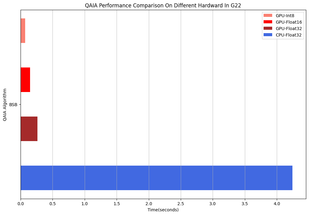
性能对比
对比BSB算法在CPU和GPU后端上求解最大割问题的性能差异
[9]:
import time

start_time = time.time()
solver = BSB(G, batch_size=100, n_iter=1000, backend="cpu-float32")
solver.update()
cut = solver.calc_cut()
cpu_time = time.time() - start_time

start_time = time.time()
solver = BSB(G, batch_size=100, n_iter=1000, backend="gpu-float32")
solver.update()
cut = solver.calc_cut()
gpu_fp32_time = time.time() - start_time

start_time = time.time()
solver = BSB(G, batch_size=100, n_iter=1000, backend="gpu-float16")
solver.update()
cut = solver.calc_cut()
gpu_fp16_time = time.time() - start_time

start_time = time.time()
solver = BSB(G, batch_size=100, n_iter=1000, backend="gpu-int8")
solver.update()
cut = solver.calc_cut()
gpu_fp8_time = time.time() - start_time
[10]:
import matplotlib.pyplot as plt

# 绘制水平条形图,表示不同后端的计算时间
plt.figure(figsize=(12, 8))
plt.barh(0.6, gpu_fp8_time, height=0.1, label="GPU-Int8", color="salmon")
plt.barh(0.4, gpu_fp16_time, height=0.1, label="GPU-Float16", color="red")
plt.barh(0.2, gpu_fp32_time, height=0.1, label="GPU-Float32", color="brown")
plt.barh(0, cpu_time, height=0.1, label="CPU-Float32", color="royalblue")

plt.title("QAIA Performance Comparison On Different Hardware In G22")
plt.xlabel("Time(seconds)")
plt.ylabel("QAIA Algorithm")
plt.yticks((0.3,), ("BSB",))

plt.grid(True, axis="x", linestyle="-", alpha=0.8)
plt.legend()
plt.show()
[11]:
from mindquantum.utils.show_info import InfoTable

InfoTable("mindquantum", "scipy", "numpy")
[11]:
| Software | Version |
|---|---|
| mindquantum | 0.10.1 |
| scipy | 1.11.3 |
| numpy | 1.26.1 |
| System | Info |
| Python | 3.10.13 |
| OS | Linux x86_64 |
| Memory | 810.22 GB |
| CPU Max Thread | 96 |
| Date | Tue Jun 10 14:55:10 2025 |