网络搭建

基础逻辑

PyTorch和MindSpore的基础逻辑如下图所示：

flowchart

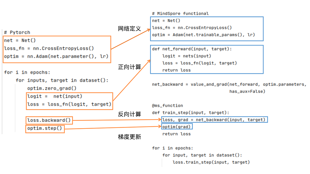
可以看到，PyTorch和MindSpore在实现流程中一般都需要网络定义、正向计算、反向计算、梯度更新等步骤。

网络定义：在网络定义中，一般会定义出需要的前向网络，损失函数和优化器。在Net()中定义前向网络，PyTorch的网络继承nn.Module；类似地，MindSpore的网络继承nn.Cell。在MindSpore中，损失函数和优化器除了使用MindSpore中提供的外，用户还可以使用自定义的优化器。可参考模型模块自定义。可以使用functional/nn等接口拼接需要的前向网络、损失函数和优化器。
正向计算：运行实例化后的网络，可以得到logit，将logit和target作为输入计算loss。需要注意的是，如果正向计算的函数有多个输出，在反向计算时需要注意多个输出对于计算结果的影响。
反向计算：得到loss后，我们可以进行反向计算。在PyTorch中可使用loss.backward()计算梯度，在MindSpore中，先用mindspore.grad()定义出反向传播方程net_backward，再将输入传入net_backward中，即可计算梯度。如果正向计算的函数有多个输出，在反向计算时，可将has_aux设置为True，即可保证只有第一个输出参与求导，其它输出值将直接返回。对于反向计算中接口用法区别详见自动微分对比。
梯度更新：将计算后的梯度更新到网络的Parameters中。在PyTorch中使用optim.step()；在MindSpore中，将Parameter的梯度传入定义好的optim中，即可完成梯度更新。

网络基本构成单元 Cell

MindSpore的网络搭建主要使用Cell进行图的构造，用户需要定义一个类继承 Cell 这个基类，在 init 里声明需要使用的API及子模块，在 construct 里进行计算， Cell 在 GRAPH_MODE (静态图模式)下将编译为一张计算图，在 PYNATIVE_MODE (动态图模式)下作为神经网络的基础模块。

PyTorchhe 和 MindSpore 基本的 Cell 搭建过程如下所示：

PyTorch

MindSpore

import torch.nn as torch_nn

class MyCell_pt(torch_nn.Module):
    def __init__(self, forward_net):
        super(MyCell_pt, self).__init__()
        self.net = forward_net
        self.relu = torch_nn.ReLU()

    def forward(self, x):
        y = self.net(x)
        return self.relu(y)

inner_net_pt = torch_nn.Conv2d(120, 240, kernel_size=4, bias=False)
pt_net = MyCell_pt(inner_net_pt)
for i in pt_net.parameters():
    print(i.shape)


运行结果：
    torch.Size([240, 120, 4, 4])

import mindspore.nn as nn
import mindspore.ops as ops

class MyCell(nn.Cell):
    def __init__(self, forward_net):
        super(MyCell, self).__init__(auto_prefix=True)
        self.net = forward_net
        self.relu = ops.ReLU()

    def construct(self, x):
        y = self.net(x)
        return self.relu(y)

inner_net = nn.Conv2d(120, 240, 4, has_bias=False)
my_net = MyCell(inner_net)
print(my_net.trainable_params())


运行结果：
[Parameter (name=net.weight, shape=(240, 120, 4, 4), dtype=Float32, requires_grad=True)]

MindSpore中，参数的名字一般是根据__init__定义的对象名字和参数定义时用的名字组成的，比如上面的例子中，卷积的参数名为net.weight，其中，net是self.net = forward_net中的对象名，weight是Conv2d中定义卷积的参数时的name：self.weight = Parameter(initializer(self.weight_init, shape), name='weight')。

MindSpore的Cell提供了auto_prefix接口用来判断Cell中的参数名是否加对象名这层信息，默认是True，也就是加对象名。如果auto_prefix设置为False，则上面这个例子中打印的Parameter的name是weight。通常骨干网络auto_prefix应设置为True。用于训练的优化器、 :class:mindspore.nn.TrainOneStepCell 等，应设置为False，以避免骨干网络的权重参数名被误改。

单元测试

有了构建Cell的脚本，需要使用相同的输入数据和参数，对输出做比较：

import numpy as np
import mindspore as ms
import torch

x = np.random.uniform(-1, 1, (2, 120, 12, 12)).astype(np.float32)
for m in pt_net.modules():
    if isinstance(m, torch_nn.Conv2d):
        torch_nn.init.constant_(m.weight, 0.1)

for _, cell in my_net.cells_and_names():
    if isinstance(cell, nn.Conv2d):
        cell.weight.set_data(ms.common.initializer.initializer(0.1, cell.weight.shape, cell.weight.dtype))

y_ms = my_net(ms.Tensor(x))
y_pt = pt_net(torch.from_numpy(x))
diff = np.max(np.abs(y_ms.asnumpy() - y_pt.detach().numpy()))
print(diff)

# ValueError: operands could not be broadcast together with shapes (2,240,12,12) (2,240,9,9)

可以发现MindSpore和PyTorch的输出不一样，什么原因呢？

查询API差异文档发现，Conv2d的默认参数在MindSpore和PyTorch上有区别， MindSpore默认使用same模式，PyTorch默认使用pad模式，迁移时需要改一下MindSpore Conv2d的pad_mode：

import numpy as np
import mindspore as ms
import torch

inner_net = nn.Conv2d(120, 240, 4, has_bias=False, pad_mode="pad")
my_net = MyCell(inner_net)

# 构造随机输入
x = np.random.uniform(-1, 1, (2, 120, 12, 12)).astype(np.float32)
for m in pt_net.modules():
    if isinstance(m, torch_nn.Conv2d):
        # 固定PyTorch初始化参数
        torch_nn.init.constant_(m.weight, 0.1)

for _, cell in my_net.cells_and_names():
    if isinstance(cell, nn.Conv2d):
        # 固定MindSpore初始化参数
        cell.weight.set_data(ms.common.initializer.initializer(0.1, cell.weight.shape, cell.weight.dtype))

y_ms = my_net(ms.Tensor(x))
y_pt = pt_net(torch.from_numpy(x))
diff = np.max(np.abs(y_ms.asnumpy() - y_pt.detach().numpy()))
print(diff)

运行结果：

2.9355288e-06

整体误差在万分之一左右，基本符合预期。在迁移Cell的过程中最好对每个Cell都做一次单元测试，保证迁移的一致性。

Cell常用的方法介绍

Cell是MindSpore中神经网络的基本构成单元，提供了很多设置标志位以及好用的方法，下面来介绍一些常用的方法。

手动混合精度

MindSpore提供了一种自动混合精度的方法，详见Model的amp_level属性。

但是有的时候开发网络时希望混合精度策略更加的灵活，MindSpore也提供了to_float的方法手动地添加混合精度。

to_float(dst_type): 在Cell和所有子Cell的输入上添加类型转换，以使用特定的浮点类型运行。

如果 dst_type 是 ms.float16 ，Cell的所有输入(包括作为常量的input， Parameter， Tensor)都会被转换为float16。

自定义的to_float和Model里的amp_level冲突，使用自定义的混合精度就不要设置Model里的amp_level。

torch.nn.Module 的 to 接口可以实现类似功能。

PyTorch和MindSpore中，将一个网络里所有的BN和loss改成float32类型，其余操作是float16类型，可以这么做：

PyTorch 设置模型数据类型

MindSpore 设置模型数据类型

import torch
import torch.nn as nn

class Network(nn.Module):
    def __init__(self):
        super(Network, self).__init__()
        self.layer1 = nn.Sequential(
            nn.Conv2d(3, 12, kernel_size=3, padding=1),
            nn.BatchNorm2d(12),
            nn.ReLU(),
            nn.MaxPool2d(kernel_size=2, stride=2)
        )
        self.layer2 = nn.Sequential(
            nn.Conv2d(12, 4, kernel_size=3, padding=1),
            nn.BatchNorm2d(4),
            nn.ReLU(),
            nn.MaxPool2d(kernel_size=2, stride=2)
        )
        self.pool = nn.AdaptiveMaxPool2d((5, 5))
        self.fc = nn.Linear(100, 10)

    def forward(self, x):
        x = self.layer1(x)
        x = self.layer2(x)
        x = self.pool(x)
        x = x.view(x.size(0), -1)
        out = self.fc(x)
        return out

net = Network()
net = net.to(torch.float32)
for name, module in net.named_modules():
    if isinstance(module, (nn.BatchNorm1d, nn.BatchNorm2d, nn.BatchNorm3d)):
        module.to(torch.float32)
loss = nn.CrossEntropyLoss(reduction='mean')
loss = loss.to(torch.float32)

import mindspore as ms
from mindspore import nn

# 定义模型
class Network(nn.Cell):
    def __init__(self):
        super().__init__()
        self.layer1 = nn.SequentialCell([
            nn.Conv2d(3, 12, kernel_size=3, pad_mode='pad', padding=1),
            nn.BatchNorm2d(12),
            nn.ReLU(),
            nn.MaxPool2d(kernel_size=2, stride=2)
        ])
        self.layer2 = nn.SequentialCell([
            nn.Conv2d(12, 4, kernel_size=3, pad_mode='pad', padding=1),
            nn.BatchNorm2d(4),
            nn.ReLU(),
            nn.MaxPool2d(kernel_size=2, stride=2)
        ])
        self.pool = nn.AdaptiveMaxPool2d((5, 5))
        self.fc = nn.Dense(100, 10)

    def construct(self, x):
        x = self.layer1(x)
        x = self.layer2(x)
        x = self.pool(x)
        x = x.view((-1, 100))
        out = nn.Dense(x)
        return out

net = Network()
net.to_float(ms.float16)  # 将net里所有的操作加float16的标志，框架会在编译时在输入加cast方法
for _, cell in net.cells_and_names():
    if isinstance(cell, (nn.BatchNorm1d, nn.BatchNorm2d, nn.BatchNorm3d)):
        cell.to_float(ms.float32)

loss = nn.SoftmaxCrossEntropyWithLogits(sparse=True, reduction='mean').to_float(ms.float32)
net_with_loss = nn.WithLossCell(net, loss_fn=loss)

Parameter管理

在 PyTorch 中，可以存储数据的对象总共有四种，分别时Tensor、Variable、Parameter、Buffer。这四种对象的默认行为均不相同，当用户不需要求梯度时，通常使用 Tensor和 Buffer两类数据对象，当用户需要求梯度时，通常使用 Variable 和 Parameter 两类对象。PyTorch 在设计这四种数据对象时，功能上存在冗余（Variable 后续会被废弃也说明了这一点）。

MindSpore 优化了数据对象的设计逻辑，仅保留了两种数据对象：Tensor 和 Parameter，其中 Tensor 对象仅参与运算，并不需要对其进行梯度求导和Parameter更新，而 Parameter 数据对象和 PyTorch 的 Parameter 意义相同，会根据其属性requires_grad 来决定是否对其进行梯度求导和Parameter更新。在网络迁移时，只要是在PyTorch中未进行Parameter更新的数据对象，均可在MindSpore中声明为 Tensor。

Parameter获取

mindspore.nn.Cell 使用 parameters_dict 、get_parameters 和 trainable_params 接口获取 Cell 中的 Parameter 。

parameters_dict：获取网络结构中所有Parameter，返回一个以key为Parameter名，value为Parameter值的OrderedDict。
get_parameters：获取网络结构中的所有Parameter，返回Cell中Parameter的迭代器。
trainable_params：获取Parameter中requires_grad为True的属性，返回可训Parameter的列表。

在定义优化器时，使用net.trainable_params()获取需要进行Parameter更新的Parameter列表。

torch.nn.Module 使用 get_parameter 、 named_parameters 、 parameters 等接口获取 Module 中的 Parameter 。

PyTorch

MindSpore

import torch.nn as nn

net = nn.Linear(2, 1)

for name, param in net.named_parameters():
    print("Parameter Name:", name)

for name, param in net.named_parameters():
    if "bias" in name:
        param.requires_grad = False

for name, param in net.named_parameters():
    if param.requires_grad:
        print("Parameter Name:", name)


运行结果：
Parameter Name: weight
Parameter Name: bias
Parameter Name: weight

import mindspore.nn as nn

net = nn.Dense(2, 1, has_bias=True)
print(net.trainable_params())

for param in net.trainable_params():
    param_name = param.name
    if "bias" in param_name:
        param.requires_grad = False
print(net.trainable_params())


运行结果：
[Parameter (name=weight, shape=(1, 2), dtype=Float32, requires_grad=True), Parameter (name=bias, shape=(1,), dtype=Float32, requires_grad=True)]
[Parameter (name=weight, shape=(1, 2), dtype=Float32, requires_grad=True)]

梯度冻结

除了使用给Parameter设置requires_grad=False来不更新Parameter外，还可以使用stop_gradient来阻断梯度计算以达到冻结Parameter的作用。那什么时候使用requires_grad=False，什么时候使用stop_gradient呢？

parameter-freeze

如上图所示，requires_grad=False不更新部分Parameter，但是反向的梯度计算还是正常执行的； stop_gradient会直接截断反向梯度，当需要冻结的Parameter之前没有需要训练的Parameter时，两者在功能上是等价的。但是stop_gradient会更快（少执行了一部分反向梯度计算）。当冻结的Parameter之前有需要训练的Parameter时，只能使用requires_grad=False。另外，stop_gradient需要加在网络的计算链路里，作用的对象是Tensor：

a = A(x)
a = ops.stop_gradient(a)
y = B(a)

Parameter保存和加载

MindSpore提供了load_checkpoint和save_checkpoint方法用来Parameter的保存和加载，需要注意的是Parameter保存时，保存的是Parameter列表，Parameter加载时对象必须是Cell。在Parameter加载时，可能Parameter名对不上需要做一些修改，可以直接构造一个新的Parameter列表给到load_checkpoint加载到Cell。

torch.nn.Module 提供 state_dict 、 load_state_dict 等接口保存加载模型的Parameter。

PyTorch

MindSpore

import torch
import torch.nn as nn

linear_layer = nn.Linear(2, 1, bias=True)

linear_layer.weight.data.fill_(1.0)
linear_layer.bias.data.zero_()

print("Original linear layer parameters:")
print(linear_layer.weight)
print(linear_layer.bias)

torch.save(linear_layer.state_dict(), 'linear_layer_params.pth')

new_linear_layer = nn.Linear(2, 1, bias=True)

new_linear_layer.load_state_dict(torch.load('linear_layer_params.pth'))

# 打印加载后的Parameter，应该和原始Parameter一样
print("Loaded linear layer parameters:")
print(new_linear_layer.weight)
print(new_linear_layer.bias)


运行结果：
Original linear layer parameters:
Parameter containing:
tensor([[1., 1.]], requires_grad=True)
Parameter containing:
tensor([0.], requires_grad=True)
Loaded linear layer parameters:
Parameter containing:
tensor([[1., 1.]], requires_grad=True)
Parameter containing:
tensor([0.], requires_grad=True)

import mindspore as ms
import mindspore.ops as ops
import mindspore.nn as nn

net = nn.Dense(2, 1, has_bias=True)
for param in net.get_parameters():
    print(param.name, param.data.asnumpy())

ms.save_checkpoint(net, "dense.ckpt")
dense_params = ms.load_checkpoint("dense.ckpt")
print(dense_params)
new_params = {}
for param_name in dense_params:
    print(param_name, dense_params[param_name].data.asnumpy())
    new_params[param_name] = ms.Parameter(ops.ones_like(dense_params[param_name].data), name=param_name)

ms.load_param_into_net(net, new_params)
for param in net.get_parameters():
    print(param.name, param.data.asnumpy())


运行结果：
weight [[-0.0042482  -0.00427286]]
bias [0.]
{'weight': Parameter (name=weight, shape=(1, 2), dtype=Float32, requires_grad=True), 'bias': Parameter (name=bias, shape=(1,), dtype=Float32, requires_grad=True)}
weight [[-0.0042482  -0.00427286]]
bias [0.]
weight [[1. 1.]]
bias [1.]

Parameter初始化

默认权重初始化不同

我们知道权重初始化对网络的训练十分重要。每个nn接口一般会有一个隐式的声明权重，在不同的框架中，隐式的声明权重可能不同。即使功能一致，隐式声明的权重初始化方式分布如果不同，也会对训练过程产生影响，甚至无法收敛。

常见隐式声明权重的nn接口：Conv、Dense(Linear)、Embedding、LSTM 等，其中区别较大的是 Conv 类和 Dense 两种接口。MindSpore和PyTorch的 Conv 类和 Dense 隐式声明的权重和偏差初始化方式分布相同。

Conv2d
- mindspore.nn.Conv2d的weight为：\(\mathcal{U} (-\sqrt{k},\sqrt{k} )\)，bias为：\(\mathcal{U} (-\sqrt{k},\sqrt{k} )\)。
- torch.nn.Conv2d的weight为：\(\mathcal{U} (-\sqrt{k},\sqrt{k} )\)，bias为：\(\mathcal{U} (-\sqrt{k},\sqrt{k} )\)。
- tf.keras.Layers.Conv2D的weight为：glorot_uniform，bias为：zeros。
其中，\(k=\frac{groups}{c_{in}*\prod_{i}^{}{kernel\_size[i]}}\)
Dense(Linear)
- mindspore.nn.Dense的weight为：\(\mathcal{U}(-\sqrt{k},\sqrt{k})\)，bias为：\(\mathcal{U}(-\sqrt{k},\sqrt{k} )\)。
- torch.nn.Linear的weight为：\(\mathcal{U}(-\sqrt{k},\sqrt{k})\)，bias为：\(\mathcal{U}(-\sqrt{k},\sqrt{k} )\)。
- tf.keras.Layers.Dense的weight为：glorot_uniform，bias为：zeros。

其中，\(k=\frac{groups}{in\_features}\) 。

对于没有正则化的网络，如没有 BatchNorm 算子的 GAN 网络，梯度很容易爆炸或者消失，权重初始化就显得十分重要，各位开发者应注意权重初始化带来的影响。

Parameter初始化API对比

每个 torch.nn.init 的API都可以和MindSpore一一对应，除了 torch.nn.init.calculate_gain() 之外。更多信息，请查看PyTorch与MindSpore API映射表。

gain 用来衡量非线性关系对于数据标准差的影响。由于非线性会影响数据的标准差，可能会导致梯度爆炸或消失。

torch.nn.init

mindspore.common.initializer

import torch

x = torch.empty(2, 2)
torch.nn.init.uniform_(x)

import mindspore
from mindspore.common.initializer import initializer, Uniform

x = initializer(Uniform(), [1, 2, 3], mindspore.float32)

mindspore.common.initializer 用于在并行模式中延迟Tensor的数据的初始化。只有在调用了 init_data() 之后，才会使用指定的 init 来初始化Tensor的数据。每个Tensor只能使用一次 init_data() 。在运行以上代码之后，x 其实尚未完成初始化。如果此时 x 被用来计算，将会作为0来处理。然而，在打印时，会自动调用 init_data() 。
torch.nn.init 需要一个Tensor作为输入，将输入的Tensor原地修改为目标结果，运行上述代码之后，x将不再是非初始化状态，其元素将服从均匀分布。

自定义初始化Parameter

MindSpore封装的高阶API里一般会给Parameter一个默认的初始化，当这个初始化分布与需要使用的初始化、PyTorch的初始化不一致，此时需要进行自定义初始化。网络参数初始化介绍了一种在使用API属性进行初始化的方法，这里介绍一种利用Cell进行Parameter初始化的方法。

Parameter的相关介绍请参考网络参数，本节主要以Cell为切入口，举例获取Cell中的所有参数，并举例说明怎样给Cell里的Parameter进行初始化。

注意本节的方法不能在construct里执行，在网络中修改Parameter的值请使用assign。

set_data(data, slice_shape=False)设置Parameter数据。

MindSpore支持的Parameter初始化方法参考mindspore.common.initializer，当然也可以直接传入一个定义好的Parameter对象。

import math
import mindspore as ms
from mindspore import nn

# 定义模型
class Network(nn.Cell):
    def __init__(self):
        super().__init__()
        self.layer1 = nn.SequentialCell([
            nn.Conv2d(3, 12, kernel_size=3, pad_mode='pad', padding=1),
            nn.BatchNorm2d(12),
            nn.ReLU(),
            nn.MaxPool2d(kernel_size=2, stride=2)
        ])
        self.layer2 = nn.SequentialCell([
            nn.Conv2d(12, 4, kernel_size=3, pad_mode='pad', padding=1),
            nn.BatchNorm2d(4),
            nn.ReLU(),
            nn.MaxPool2d(kernel_size=2, stride=2)
        ])
        self.pool = nn.AdaptiveMaxPool2d((5, 5))
        self.fc = nn.Dense(100, 10)

    def construct(self, x):
        x = self.layer1(x)
        x = self.layer2(x)
        x = self.pool(x)
        x = x.view((-1, 100))
        out = nn.Dense(x)
        return out

net = Network()
for _, cell in net.cells_and_names():
    if isinstance(cell, nn.Conv2d):
        cell.weight.set_data(ms.common.initializer.initializer(
            ms.common.initializer.HeNormal(negative_slope=0, mode='fan_out', nonlinearity='relu'),
            cell.weight.shape, cell.weight.dtype))
    elif isinstance(cell, (nn.BatchNorm2d, nn.GroupNorm)):
        cell.gamma.set_data(ms.common.initializer.initializer("ones", cell.gamma.shape, cell.gamma.dtype))
        cell.beta.set_data(ms.common.initializer.initializer("zeros", cell.beta.shape, cell.beta.dtype))
    elif isinstance(cell, (nn.Dense)):
        cell.weight.set_data(ms.common.initializer.initializer(
            ms.common.initializer.HeUniform(negative_slope=math.sqrt(5)),
            cell.weight.shape, cell.weight.dtype))
        cell.bias.set_data(ms.common.initializer.initializer("zeros", cell.bias.shape, cell.bias.dtype))

子模块管理

mindspore.nn.Cell 中可定义其他Cell实例作为子模块。这些子模块是网络中的组成部分，自身也可能包含可学习的Parameter（如卷积层的权重和偏置）和其他子模块。这种层次化的模块结构允许用户构建复杂且可重用的神经网络架构。

mindspore.nn.Cell 提供 cells_and_names 、 insert_child_to_cell 等接口实现子模块管理功能。

torch.nn.Module 提供 named_modules 、 add_module 等接口实现子模块管理功能。

PyTorch

MindSpore

import torch.nn as nn

class MyModule(nn.Module):
    def __init__(self):
        super(MyModule, self).__init__()
        self.conv1 = nn.Conv2d(1, 32, 3, 1)
        self.conv2 = nn.Conv2d(32, 64, 3, 1)
        # 使用add_module添加子模块
        self.add_module('conv3', nn.Conv2d(64, 128, 3, 1))

        self.sequential_block = nn.Sequential(
            nn.ReLU(),
            nn.Conv2d(128, 256, 3, 1),
            nn.ReLU()
        )

    def forward(self, x):
        x = self.conv1(x)
        x = self.conv2(x)
        x = self.conv3(x)
        x = self.sequential_block(x)
        return x

module = MyModule()

# 使用named_modules遍历所有子模块（包括直接和间接子模块）
for name, module_instance in module.named_modules():
    print(f"Module name: {name}, type: {type(module_instance)}")


运行结果：
Module name: , type: <class '__main__.MyModule'>
Module name: conv1, type: <class 'torch.nn.modules.conv.Conv2d'>
Module name: conv2, type: <class 'torch.nn.modules.conv.Conv2d'>
Module name: conv3, type: <class 'torch.nn.modules.conv.Conv2d'>
Module name: sequential_block, type: <class 'torch.nn.modules.container.Sequential'>
Module name: sequential_block.0, type: <class 'torch.nn.modules.activation.ReLU'>
Module name: sequential_block.1, type: <class 'torch.nn.modules.conv.Conv2d'>
Module name: sequential_block.2, type: <class 'torch.nn.modules.activation.ReLU'>

from mindspore import nn

class MyCell(nn.Cell):
    def __init__(self):
        super(MyCell, self).__init__()
        self.conv1 = nn.Conv2d(1, 32, 3, 1)
        self.conv2 = nn.Conv2d(32, 64, 3, 1)
        # 使用insert_child_to_cell添加子模块
        self.insert_child_to_cell('conv3', nn.Conv2d(64, 128, 3, 1))

        self.sequential_block = nn.SequentialCell(
            nn.ReLU(),
            nn.Conv2d(128, 256, 3, 1),
            nn.ReLU()
        )

    def construct(self, x):
        x = self.conv1(x)
        x = self.conv2(x)
        x = self.conv3(x)
        x = self.sequential_block(x)
        return x

module = MyCell()

# 使用cells_and_names遍历所有子模块（包括直接和间接子模块）
for name, cell_instance in module.cells_and_names():
    print(f"Cell name: {name}, type: {type(cell_instance)}")


运行结果：
Cell name: , type: <class '__main__.MyCell'>
Cell name: conv1, type: <class 'mindspore.nn.layer.conv.Conv2d'>
Cell name: conv2, type: <class 'mindspore.nn.layer.conv.Conv2d'>
Cell name: conv3, type: <class 'mindspore.nn.layer.conv.Conv2d'>
Cell name: sequential_block, type: <class 'mindspore.nn.layer.container.SequentialCell'>
Cell name: sequential_block.0, type: <class 'mindspore.nn.layer.activation.ReLU'>
Cell name: sequential_block.1, type: <class 'mindspore.nn.layer.conv.Conv2d'>
Cell name: sequential_block.2, type: <class 'mindspore.nn.layer.activation.ReLU'>

训练评估模式切换

torch.nn.Module 提供 train(mode=True) 接口设置模型处于训练模式和 eval 接口设置模型处于评估模式。这两种模式的区别主要体现在Dropout和BN等层的行为以及权重更新上。

Dropout和BN层的行为：

训练模式下，Dropout层会按照设定的Parameter p 来随机关闭一部分神经元，这意味着在前向传播过程中，这部分神经元不会有任何贡献。BN层会继续计算均值和方差，并对数据进行相应的归一化。

评估模式下，Dropout层不会关闭任何神经元，即所有的神经元都会被用于前向传播。BN层会使用训练阶段计算得到的运行均值和运行方差。
权重更新：

在训练模式下，模型的权重会根据反向传播的结果进行更新。这意味着在每次前向传播和反向传播之后，模型的权重都可能会发生变化。

在评估模式下，模型的权重不会被更新。即使进行了前向传播并计算了损失，也不会进行反向传播来更新权重。这是因为评估模式主要用于测试模型的性能，而不是训练模型。

mindspore.nn.Cell 提供 set_train(mode=True) 接口实现模式的切换。mode 设置成 True 时，模型处于训练模式；mode 设置成 False 时，模型处于评估模式。

设备相关

torch.nn.Module 提供 CPU 、 cuda 、 ipu 等接口将模型移动到指定设备上。

mindspore.set_context() 的 device_target 参数实现类似功能， device_target 可以指定 CPU 、 GPU 和 Ascend 设备。与PyTorch不同的是，一旦设备设置成功，输入数据和模型会默认拷贝到指定的设备中执行，不需要也无法再改变数据和模型所运行的设备类型。

PyTorch

MindSpore

import torch
torch_net = torch.nn.Linear(3, 4)
torch_net.cpu()

import mindspore
mindspore.set_context(device_target="CPU")
ms_net = mindspore.nn.Dense(3, 4)

动态图与静态图

对于Cell，MindSpore提供GRAPH_MODE（静态图）和PYNATIVE_MODE（动态图）两种模式，详情请参考动态图和静态图。

PyNative模式下模型进行推理的行为与一般Python代码无异。但是在训练过程中，注意一旦将Tensor转换成numpy做其他的运算后将会截断网络的梯度，相当于PyTorch的detach。

而在使用GRAPH_MODE时，通常会出现语法限制。在这种情况下，需要对Python代码进行图编译操作，而这一步操作中MindSpore目前还未能支持完整的Python语法全集，所以construct函数的编写会存在部分限制。具体限制内容可以参考MindSpore静态图语法。

相较于详细的语法说明，常见的限制可以归结为以下几点：

场景1

限制：构图时（construct函数部分或者用@jit修饰的函数），不要调用其他Python库，例如numpy、scipy，相关的处理应该前移到__init__阶段。措施：使用MindSpore内部提供的API替换其他Python库的功能。常量的处理可以前移到__init__阶段。
场景2

限制：构图时不要使用自定义类型，而应该使用MindSpore提供的数据类型和Python基础类型，可以使用基于这些类型的tuple/list组合。措施：使用基础类型进行组合，可以考虑增加函数参数量。函数入参数没有限制，并且可以使用不定长输入。
场景3

限制：构图时不要对数据进行多线程或多进程处理。措施：避免网络中出现多线程处理。

自定义反向

但是有的时候MindSpore不支持某些处理，需要使用一些三方的库的方法，但是我们又不想截断网络的梯度，这时该怎么办呢？这里介绍一种在PYNATIVE_MODE模式下，通过自定义反向规避此问题的方法：

有这么一个场景，需要随机有放回的选取大于0.5的值，且每个batch的shape固定是max_num。但是这个随机有放回的操作目前没有MindSpore的API支持，这时我们在PYNATIVE_MODE下使用numpy的方法来计算，然后自己构造一个梯度传播的过程。

import numpy as np
import mindspore as ms
import mindspore.nn as nn
import mindspore.ops as ops

ms.set_context(mode=ms.PYNATIVE_MODE)
ms.set_seed(1)

class MySampler(nn.Cell):
    # 自定义取样器，在每个batch选取max_num个大于0.5的值
    def __init__(self, max_num):
        super(MySampler, self).__init__()
        self.max_num = max_num

    def random_positive(self, x):
        # 三方库numpy的方法，选取大于0.5的位置
        pos = np.where(x > 0.5)[0]
        pos_indice = np.random.choice(pos, self.max_num)
        return pos_indice

    def construct(self, x):
        # 正向网络构造
        batch = x.shape[0]
        pos_value = []
        pos_indice = []
        for i in range(batch):
            a = x[i].asnumpy()
            pos_ind = self.random_positive(a)
            pos_value.append(ms.Tensor(a[pos_ind], ms.float32))
            pos_indice.append(ms.Tensor(pos_ind, ms.int32))
        pos_values = ops.stack(pos_value, axis=0)
        pos_indices = ops.stack(pos_indice, axis=0)
        print("pos_values forword", pos_values)
        print("pos_indices forword", pos_indices)
        return pos_values, pos_indices

x = ms.Tensor(np.random.uniform(0, 3, (2, 5)), ms.float32)
print("x", x)
sampler = MySampler(3)
pos_values, pos_indices = sampler(x)
grad = ms.grad(sampler, grad_position=0)(x)
print("dx", grad)

运行结果：

x [[1.2510660e+00 2.1609735e+00 3.4312444e-04 9.0699774e-01 4.4026768e-01]
 [2.7701578e-01 5.5878061e-01 1.0366821e+00 1.1903024e+00 1.6164502e+00]]
pos_values forword [[0.90699774 2.1609735  0.90699774]
 [0.5587806  1.6164502  0.5587806 ]]
pos_indices forword [[3 1 3]
 [1 4 1]]
pos_values forword [[0.90699774 1.251066   2.1609735 ]
 [1.1903024  1.1903024  0.5587806 ]]
pos_indices forword [[3 0 1]
 [3 3 1]]
dx (Tensor(shape=[2, 5], dtype=Float32, value=
[[0.00000000e+000, 0.00000000e+000, 0.00000000e+000, 0.00000000e+000, 0.00000000e+000],
 [0.00000000e+000, 0.00000000e+000, 0.00000000e+000, 0.00000000e+000, 0.00000000e+000]]),)

当我们不构造这个反向过程时，由于使用的是numpy的方法计算的pos_value，梯度将会截断。如上面注释所示，dx的值全是0。另外细心的同学会发现这个过程打印了两次pos_values forword和pos_indices forword，这是因为在PYNATIVE_MODE下在构造反向图时会再次构造一次正向图，这使得上面的这种写法实际上跑了两次正向和一次反向，这不但浪费了训练资源，在某些情况还会造成精度问题，如有BatchNorm的情况，在运行正向时就会更新moving_mean和moving_var导致一次训练更新了两次moving_mean和moving_var。为了避免这种场景，MindSpore针对Cell有一个方法set_grad()，在PYNATIVE_MODE模式下框架会在构造正向时同步构造反向，这样在执行反向时就不会再运行正向的流程了。

x = ms.Tensor(np.random.uniform(0, 3, (2, 5)), ms.float32)
print("x", x)
sampler = MySampler(3).set_grad()
pos_values, pos_indices = sampler(x)
grad = ms.grad(sampler, grad_position=0)(x)
print("dx", grad)

运行结果：

x [[1.2519144  1.6760695  0.42116082 0.59430444 2.4022336 ]
 [2.9047847  0.9402725  2.076968   2.6291676  2.68382   ]]
pos_values forword [[1.2519144 1.2519144 1.6760695]
 [2.6291676 2.076968  0.9402725]]
pos_indices forword [[0 0 1]
 [3 2 1]]
dx (Tensor(shape=[2, 5], dtype=Float32, value=
[[0.00000000e+000, 0.00000000e+000, 0.00000000e+000, 0.00000000e+000, 0.00000000e+000],
 [0.00000000e+000, 0.00000000e+000, 0.00000000e+000, 0.00000000e+000, 0.00000000e+000]]),)

下面，我们来演示下如何自定义反向：

import numpy as np
import mindspore as ms
import mindspore.nn as nn
import mindspore.ops as ops

ms.set_context(mode=ms.PYNATIVE_MODE)
ms.set_seed(1)

class MySampler(nn.Cell):
    # 自定义取样器，在每个batch选取max_num个大于0.5的值
    def __init__(self, max_num):
        super(MySampler, self).__init__()
        self.max_num = max_num

    def random_positive(self, x):
        # 三方库numpy的方法，选取大于0.5的位置
        pos = np.where(x > 0.5)[0]
        pos_indice = np.random.choice(pos, self.max_num)
        return pos_indice

    def construct(self, x):
        # 正向网络构造
        batch = x.shape[0]
        pos_value = []
        pos_indice = []
        for i in range(batch):
            a = x[i].asnumpy()
            pos_ind = self.random_positive(a)
            pos_value.append(ms.Tensor(a[pos_ind], ms.float32))
            pos_indice.append(ms.Tensor(pos_ind, ms.int32))
        pos_values = ops.stack(pos_value, axis=0)
        pos_indices = ops.stack(pos_indice, axis=0)
        print("pos_values forword", pos_values)
        print("pos_indices forword", pos_indices)
        return pos_values, pos_indices

    def bprop(self, x, out, dout):
        # 反向网络构造
        pos_indices = out[1]
        print("pos_indices backward", pos_indices)
        grad_x = dout[0]
        print("grad_x backward", grad_x)
        batch = x.shape[0]
        dx = []
        for i in range(batch):
            dx.append(ops.UnsortedSegmentSum()(grad_x[i], pos_indices[i], x.shape[1]))
        return ops.stack(dx, axis=0)

x = ms.Tensor(np.random.uniform(0, 3, (2, 5)), ms.float32)
print("x", x)
sampler = MySampler(3).set_grad()
pos_values, pos_indices = sampler(x)
grad = ms.grad(sampler, grad_position=0)(x)
print("dx", grad)

运行结果：

x [[1.2510660e+00 2.1609735e+00 3.4312444e-04 9.0699774e-01 4.4026768e-01]
 [2.7701578e-01 5.5878061e-01 1.0366821e+00 1.1903024e+00 1.6164502e+00]]
pos_values forword [[0.90699774 2.1609735  0.90699774]
 [0.5587806  1.6164502  0.5587806 ]]
pos_indices forword [[3 1 3]
 [1 4 1]]
pos_indices backward [[3 1 3]
 [1 4 1]]
grad_x backward [[1. 1. 1.]
 [1. 1. 1.]]
dx (Tensor(shape=[2, 5], dtype=Float32, value=
[[0.00000000e+000, 1.00000000e+000, 0.00000000e+000, 2.00000000e+000, 0.00000000e+000],
 [0.00000000e+000, 2.00000000e+000, 0.00000000e+000, 0.00000000e+000, 1.00000000e+000]]),)

我们在MySampler类里加入了bprop方法，这个方法的输入是正向的输入（展开写），正向的输出（一个tuple），输出的梯度（一个tuple）。在这个方法里构造梯度到输入的梯度反传流程。可以看到在第0个batch，我们随机选取第3、1、3位置的值，输出的梯度都是1，最后反传出去的梯度为[0.00000000e+000, 1.00000000e+000, 0.00000000e+000, 2.00000000e+000, 0.00000000e+000]，符合预期。

动态shape规避策略

一般动态shape引入的原因有：

输入shape不固定；
网络执行过程中有引发shape变化的算子；
控制流不同分支引入shape上的变化。

下面，我们针对这几种场景介绍一些规避策略。

输入shape不固定的场景

可以在输入数据上加pad，pad到固定的shape。如deep_speechv2的数据处理规定input_length的最大长度，短的补0，长的随机截断，但是注意这种方法可能会影响训练的精度，需要平衡训练精度和训练性能。
可以设置一组固定的输入shape，将输入分别处理成几个固定的尺度。如YOLOv3_darknet53的数据处理，在batch方法加处理函数multi_scale_trans,在其中在MultiScaleTrans中随机选取一个shape进行处理。

目前对输入shape完全随机的情况支持有限，需要等待新版本支持。

网络执行过程中有引发shape变化的操作

对于网络运行过程中生成不固定shape的Tensor的场景，最常用的方式是构造mask来过滤掉无效的位置的值。一个简单的例子，在检测场景下需要根据预测框和真实框的iou结果选取一些框。 PyTorch 和 MindSpore（MindSpore1.8之后全场景支持了masked_select）的实现方式如下：

PyTorch

MindSpore

def box_select_torch(box, iou_score):
    mask = iou_score > 0.3
    return box[mask]

import mindspore as ms
from mindspore import ops

ms.set_seed(1)

def box_select_ms(box, iou_score):
    mask = (iou_score > 0.3).expand_dims(1)
    return ops.masked_select(box, mask)

看一下结果对比：

import torch
import numpy as np
import mindspore as ms

ms.set_seed(1)

box = np.random.uniform(0, 1, (3, 4)).astype(np.float32)
iou_score = np.random.uniform(0, 1, (3,)).astype(np.float32)

print("box_select_ms", box_select_ms(ms.Tensor(box), ms.Tensor(iou_score)))
print("box_select_torch", box_select_torch(torch.from_numpy(box), torch.from_numpy(iou_score)))

运行结果：

box_select_ms [0.14675589 0.09233859 0.18626021 0.34556073]
box_select_torch tensor([[0.1468, 0.0923, 0.1863, 0.3456]])

但是这样操作后会产生动态shape，在后续的网络计算中可能会有问题，在现阶段，推荐先使用mask规避一下：

def box_select_ms2(box, iou_score):
    mask = (iou_score > 0.3).expand_dims(1)
    return box * mask, mask

在后续计算中，如果涉及box的一些操作，需要注意是否需要乘mask用来过滤非有效结果。

对于求loss时对feature做选取，导致获取到不固定shape的Tensor的场景，处理方式基本和网络运行过程中不固定shape的处理方式相同，只是loss部分后续可能没有其他的操作，不需要返回mask。

举个例子，我们想选取前70%的正样本的值求loss。实现如下：

PyTorch

MindSpore

import torch
import torch.nn as torch_nn

class ClassLoss_pt(torch_nn.Module):
    def __init__(self):
        super(ClassLoss_pt, self).__init__()
        self.con_loss = torch_nn.CrossEntropyLoss(reduction='none')

    # 使用 torch.topk 来获取前70%的正样本数据
    def forward(self, pred, label):
        mask = label > 0
        vaild_label = label * mask
        pos_num = torch.clamp(mask.sum() * 0.7, 1).int()
        con = self.con_loss(pred, vaild_label.long()) * mask
        loss, unused_value = torch.topk(con, k=pos_num)
        return loss.mean()

import mindspore as ms
from mindspore import ops
from mindspore import nn as ms_nn
class ClassLoss_ms(ms_nn.Cell):
    def __init__(self):
        super(ClassLoss_ms, self).__init__()
        self.con_loss = ms_nn.SoftmaxCrossEntropyWithLogits(sparse=True, reduction="none")
        self.sort_descending = ops.Sort(descending=True)
    # MindSpore目前不支持TopK的K是变量，转换思路，获取到第K大的值，然后通过该值获取到topk的mask
    def construct(self, pred, label):
        mask = label > 0
        vaild_label = label * mask
        pos_num = ops.maximum(mask.sum() * 0.7, 1).astype(ms.int32)
        con = self.con_loss(pred, vaild_label.astype(ms.int32)) * mask
        con_sort, unused_value = self.sort_descending(con)
        con_k = con_sort[pos_num - 1]
        con_mask = (con >= con_k).astype(con.dtype)
        loss = con * con_mask
        return loss.sum() / con_mask.sum()

我们来看一下实验结果：

import torch
import numpy as np
import mindspore as ms
ms.set_seed(1)

pred = np.random.uniform(0, 1, (5, 2)).astype(np.float32)
label = np.array([-1, 0, 1, 1, 0]).astype(np.int32)
print("pred", pred)
print("label", label)
t_loss = ClassLoss_pt()
cls_loss_pt = t_loss(torch.from_numpy(pred), torch.from_numpy(label))
print("cls_loss_pt", cls_loss_pt)
m_loss = ClassLoss_ms()
cls_loss_ms = m_loss(ms.Tensor(pred), ms.Tensor(label))
print("cls_loss_ms", cls_loss_ms)

运行结果：

pred [[4.17021990e-01 7.20324516e-01]
 [1.14374816e-04 3.02332580e-01]
 [1.46755889e-01 9.23385918e-02]
 [1.86260208e-01 3.45560730e-01]
 [3.96767467e-01 5.38816750e-01]]
label [-1  0  1  1  0]
cls_loss_pt tensor(0.7207)
cls_loss_ms 0.7207259

控制流不同分支引入shape上的变化

分析下在模型分析与准备章节的例子：

import numpy as np
import mindspore as ms
from mindspore import ops
np.random.seed(1)
x = ms.Tensor(np.random.uniform(0, 1, (10)).astype(np.float32))
cond = (x > 0.5).any()

if cond:
    y = ops.masked_select(x, x > 0.5)
else:
    y = ops.zeros_like(x)
print(x)
print(cond)
print(y)

运行结果：

[4.17021990e-01 7.20324516e-01 1.14374816e-04 3.02332580e-01
 1.46755889e-01 9.23385918e-02 1.86260208e-01 3.45560730e-01
 3.96767467e-01 5.38816750e-01]
True
[0.7203245  0.53881675]

在cond=True时，最大的shape和x一样大，根据上面的加mask方法，可以写成：

import numpy as np
import mindspore as ms
from mindspore import ops
np.random.seed(1)
x = ms.Tensor(np.random.uniform(0, 1, (10)).astype(np.float32))
cond = (x > 0.5).any()

if cond:
    mask = (x > 0.5).astype(x.dtype)
else:
    mask = ops.zeros_like(x)
y = x * mask
print(x)
print(cond)
print(y)

运行结果：

[4.17021990e-01 7.20324516e-01 1.14374816e-04 3.02332580e-01
 1.46755889e-01 9.23385918e-02 1.86260208e-01 3.45560730e-01
 3.96767467e-01 5.38816750e-01]
True
[0.         0.7203245  0.         0.         0.         0.
 0.         0.         0.         0.53881675]

需要注意的是如果y在后续有参与其他的计算，需要一起传入mask对有效位置做过滤。

随机数策略对比

随机数API对比

PyTorch与MindSpore在接口名称上无差异，MindSpore由于不支持原地修改，所以缺少Tensor.random_接口。其余接口均可和PyTorch一一对应。

随机种子和生成器

MindSpore使用seed控制随机数的生成，而PyTorch使用torch.Generator进行随机数的控制。

MindSpore的seed分为两个等级，graph-level和op-level。graph-level下seed作为全局变量，绝大多数情况下无需用户设置，用户只需调整op-level seed。（API中涉及的seed参数，均为op-level）如果一段程序中两次使用了同一个随机数算法，那么两次的结果是不同的（尽管设置了相同的随机种子）；如果重新运行脚本，那么第二次运行的结果应该与第一次保持一致。示例如下：

# If a random op is called twice within one program, the two results will be different:
import mindspore as ms
from mindspore import Tensor, ops

minval = Tensor(1.0, ms.float32)
maxval = Tensor(2.0, ms.float32)
print(ops.uniform((1, 4), minval, maxval, seed=1))  # generates 'A1'
print(ops.uniform((1, 4), minval, maxval, seed=1))  # generates 'A2'
# If the same program runs again, it repeat the results:
print(ops.uniform((1, 4), minval, maxval, seed=1))  # generates 'A1'
print(ops.uniform((1, 4), minval, maxval, seed=1))  # generates 'A2'

torch.Generator常在函数中作为关键字参数传入。在未指定/实例化Generator时，会使用默认Generator (torch.default_generator)。可以使用以下代码设置指定的torch.Generator的seed：
```
G = torch.Generator()
G.manual_seed(1)
```
此时和使用default_generator并将seed设置为1的结果相同。例如torch.manual_seed(1)。

PyTorch的Generator中的state表示的是此Generator的状态，长度为5056，dtype为uint8的Tensor。在同一个脚本中，多次使用同一个Generator，Generator的state会发生改变。在有两个/多个Generator的情况下，如g1，g2，可以设置 g2.set_state(g1.get_state()) 使得g2达到和g1相同的状态。即使用g2相当于使用当时状态的g1。如果g1和g2具有相同的seed和state，则二者生成的随机数相同。