Automatic Parallel Strategy Search
![]()
The auto-parallel mode allows the user to automatically build the cost model and find a parallel strategy with shorter training time without paying attention to the strategy configuration. Currently MindSpore supports the following two different auto-parallel schemes:
Sharding Strategy Propagation Algorithm: propagation of parallel strategy from operators configured with parallel strategy to operators not configured. When propagating, the algorithm tries to pick the strategy that triggers the least amount of tensor rearranging communication.
Double Recursive Strategy Search Algorithm: Its cost model based on symbolic operations can be freely adapted to different accelerator clusters, and can generate optimal strategy fast for huge networks and large-scale multi-card slicing.
Automatic Parallel Strategy Search is the strategy search algorithm based on the operator-level model parallel, and to understand the principles, it is first necessary to understand the basic concepts in MindSpore operator-level parallel: distributed operators, tensor arranging, and tensor rearranging. Operator-level parallel is an implementation of Single Program Multiple Data (SPMD). The same program is executed on different data slices.
MindSpore converts a stand-alone version of a program into a parallel version. The conversion is fine-grained, replacing each operator in the stand-alone version of the program with a distributed operator, while ensuring that the replacement is mathematically equivalent.
Distributed Operators
Distributed operators running on multiple devices guarantees computational semantic equivalence with the stand-alone version of the operator. That is: given the same input, the distributed operator always gets the same output as that of the stand-alone version.
Taking the matrix multiplication operator (MatMul) as an example, inputs are two matrices X and W and output is Y = MatMul(X, W). Suppose that this operator is sliced to be executed in parallel on four devices, the exact implementation depends on the sharding strategy of the input matrices:
Case 1: If the matrix X has copies on all 4 devices, and W is sliced by column into 4 copies, one for each device, then the distributed operator corresponding to the stand-alone version of the MatMul operator is also MatMul; i.e., the MatMul operator will be executed on each device.
Case 2: If X is sliced into 4 parts according to columns and W is sliced into 4 parts according to rows, and each machine gets one slice of X and W each, then the distributed operator corresponding to the single-machine version of the MatMul operator is MatMul->AllReduce; that is, the two operators MatMul and AllReduce will be executed sequentially on each device in order to ensure mathematical equivalence.
In addition to Single Program (SP), Multiple Data (MD) also needs to be specified, i.e., the device is specified to get one slice of the data. To do this, we first define the sharding strategy.
Tensor Arrangement
Given a sharding strategy for an operator, a tensor arrangement that can derive the input and output tensors of that operator. Tensor arrangement is composed of a logical device matrix and a tensor mapping:
The logical device matrix, which is shared by the input and output tensor of this operator, is a one-dimensional array representing how the devices are organized.
The tensor mapping is a two-dimensional array that represents a dimension of the tensor sliced into a dimension of the logical device matrix.
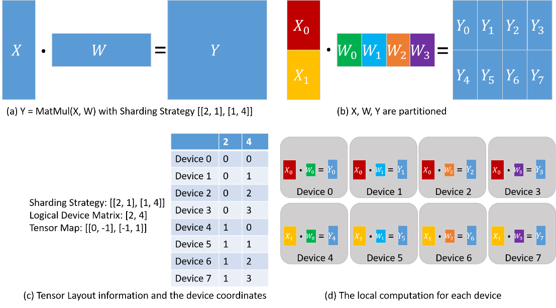
Taking the matrix multiplication operator (MatMul) as an example, its inputs are two matrices X and W, and the output is Y = MatMul(X, W). Configure the operator with a sharding strategy of [[2, 1], [1, 4]], and the obtained tensor arrangement and computations performed on each device are shown below. X is uniformly sliced into 2 parts along the rows, and W is uniformly sliced into 4 parts along the columns (Figure (b) below). Based on the sharding strategy, the logical device matrix and tensor mapping are derived as shown in Figure (c) below. The coordinates of the individual devices are thus determined, describing their positions in the logical device matrix. The distribution of the tensor in each device is determined by the coordinates of the device. From column '2' of the table in figure (c) below: device 0-device 3 get \(X_0\) slice, device 4-device 7 get \(X_1\) slice. From column '4' of the table in figure (c) below: device 0 and device 4 get \(W_0\) slice, device 1 and device 5 get \(W_1\) slice, device 2 and device 6 get \(W_2\) slice, device 3 and device 7 get \(W_3\) Slicing. Therefore, the calculations on each device are also determined as shown in figure (d) below.
For two operators with data dependency (i.e., the output tensor of one operator is used by the second operator), the tensor arrangement defined by the two operators for that data-dependent tensor may be different (due to different logical device matrices or different tensor mappings), and thus tensor rearrangement is proposed to convert the inconsistent arrangement. The definition of tensor rearrangement is given here and the specific algorithm is omitted.
Tensor Rearrangement
Given two inconsistent tensor arrangements of the same tensor, tensor rearrangement is able to convert the source arrangement to the destination arrangement while ensuring that the communication cost incurred by the conversion is minimized. The communication cost here refers to the amount of data communicated by each device.
Taking two matrix multiplication operators as an example: Z = MatMul(X, W), O = MatMul(Z, Y). In order to make the tensor rearrangement work, the two matrix multiplication operators are configured with different sharding strategies that make the arrangement of tensor Z inconsistent. In the figure (a) below, the output tensor Z of the first matrix multiplication operator is sliced by rows, however, the second matrix multiplication operator requires the tensor Z to be complete, so the tensor rearrangement infers that the AllGather operator needs to be inserted here to complete the conversion [1]. In figure (b) below, the output tensor Z of the first matrix multiplication operator is sliced by rows, however, the second matrix multiplication operator requires that the tensor Z is sliced by columns, so the tensor rearrangement deduces that the AllToAll operator needs to be inserted here to complete the conversion.
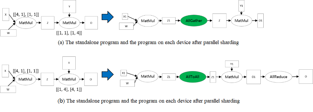
[1] Note: The AllGather operator and the Concat operator actually need to be inserted.
Strategy Propagation Algorithm
Sharding Strategy Propagation Algorithm
The sharding strategy propagation algorithm means that the user only needs to manually define the strategies for a few key operators, and the strategies for the rest of the operators in the computation graph are automatically generated by the algorithm. Because the strategies of the key operators have been defined, the cost model of the algorithm mainly describes the redistribution cost between operators, and the optimization objective is to minimize the cost of the whole graph redistribution. Because the main operator strategy has been defined, which is equivalent to compress the search space, the search time of this scheme is shorter, and its strategy performance relies on the definition of the key operator strategy, so it still requires the user to have some ability to analyze the definition strategy.
Hardware platforms supported by the sharding strategy propagation algorithm include Ascend, in addition to both PyNative mode and Graph mode.
Related interfaces:
mindspore.parallel.auto_parallel.AutoParallel(net, parallel_mode="sharding_propagation"): Set the parallel mode and select the Strategy Propagation Algorithm via
parallel_mode.mindspore.nn.Cell.shard() and mindspore.ops.Primitive.shard(): Specifies the operator sharding strategy, and the strategy for the rest of the operators is derived by the propagation algorithm. Currently the
mindspore.nn.Cell.shard()interface can be used in PyNative mode and Graph mode; Themindspore.ops.Primitive.shard()interface can only be used in Graph mode.
In summary, the sharding strategy propagation algorithm requires the user to manually configure the sharding strategy of the key operator.
Basic Principles
Given a computation graph, Sharding Propagation is a functionality that propagates the Sharding Strategies from configured operator to the whole graph, with the goal of minimizing the communication cost in Tensor Redistribution.
The input to the sharding strategy propagation is a computational graph with some operator sharding strategy, where points denote operators and directed edges denote data dependencies. Sharding Propagation executes as follows:
Generate possible Sharding Strategies for non-configured operators;
Generate Tensor Redistributions and the associated communication costs for each edge;
Start from the configured operators, and propagate the Sharding Strategies to non-configured operators using BFS, with the goal of minimizing the communication cost along each edge.
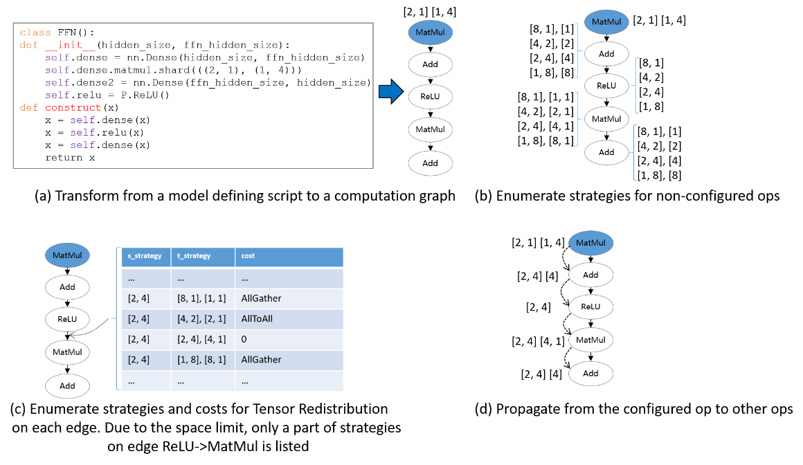
The following figure illustrates an example process of applying Sharding Propagation:
Given an computation graph with some configured strategies, it first enumerates possible strategies for non-configured operators, as shown in figure (b).
Next, it enumerates possible strategies and the Tensor Redistribution costs for each edge. Demonstrated in figure (c), the strategy for an edge is defined as a pair [s_strategy, t_strategy], where s_strategy and t_strategy denote Sharding Strategy for source operator and target operator, respectively.
Finally, starting from the configured operator, it determines the next operator's Sharding Strategy, such that the communication cost in Tensor Redistribution is minimized. The propagation ends when the Sharding Strategies for all operators are settled, as shown in figure (d).
Double Recursive Strategy Search Algorithm
The double recursive strategy search algorithm is based on Symbolic Automatic Parallel Planner (SAPP). The SAPP algorithm is able to quickly generate a communication-efficient strategy for huge neural networks. The cost model compares the relative costs of different parallel strategy rather than the predicted absolute delay, thus greatly compressing the search space and guaranteeing minute-level search times for 100-card clusters.
Hardware platforms supported by the double recursive strategy search algorithm include Ascend, and need to run in Graph mode.
Related interfaces: mindspore.parallel.auto_parallel.AutoParallel(net, parallel_mode="recursive_programming"): Set the parallel mode to auto-parallel and the search mode to a double recursive strategy search algorithm. For typical models, which have at least one operator for which recursive has a cost model (see list below), no additional configuration is required for the double recursive strategy search algorithm, except for the AutoParallel above.
Basic Principles
The double recursive strategy search algorithm is a fully automatic operator-level strategy search scheme, where the user does not need to configure a typical model in any way, and the algorithm automatically searches for parallel policies that minimize the communication cost.
There are two core shortcomings of traditional automatic operator-level strategy search.
The exponential slicing entails a large search space and traversing these potential search space is time-consuming.
It is necessary to conduct profiling in order to construct cost model and analyze different sharding strategies. However, profiling and analyzing profiling results will cost extra time.
For the first problem, the double recursive strategy search algorithm summarizes its symmetric multi-order characteristics by abstracting the AI training cluster, so it can equivalently perform a recursive dichotomy to compress the search space due to the number of devices; on the other hand, the double recursive strategy search algorithm categorizes the communication cost of operators, compares the communication cost within the operators as well as the cost of rearrangement of the operators, and compresses the exponentially complex search complexity to a linear one by ranking the weights of the operators.
For the second problem, the double recursive strategy search algorithm builds a symbolic cost model, whereas the cost model of the traditional approach focuses on how to accurately predict the absolute delay of different strategies. The cost model of the double recursive strategy search algorithm compares the relative cost of different strategies, and thus saves significantly the cost of profiling.
Therefore, the double recursive strategy search algorithm is able to quickly generate optimal strategies for huge networks and large-scale cluster slicing. In summary, the double recursive strategy search algorithm is modeled based on the parallel principle, describes the hardware cluster topology by building an abstract machine, and simplifies the cost model by symbolization. Its cost model compares not the predicted absolute latency, but the relative cost of different parallel strategies, which can greatly compress the search space and guarantee minute-level search times for 100-card clusters.
The double recursive algorithm works in two main phases:
For operators which double recursive has a cost model, their parallel strategies is automatically generated
Strategy propagation is then used to generate the strategies of other operators using previously generated strategies
For double recursive to generate strategies, there must be at least one operator with a cost model in the network, or an initial strategy set by SAPP interfered. Otherwise the propagation can not generate strategies and all operators will have a replicated parallel strategy by default.
The list of operators which have a cost model includes:
MatMul
BatchMatMul
Convolution (Conv2D, Conv2DTranspose)
Pooling ops (Pooling, MaxPool, MaxPoolV2)
BatchNorm
PReLU
UnsortedSegment ops (UnsortedSegmentSum, UnsortedSegmentMin, UnsortedSegmentMax)
SoftmaxCrossEntropyWithLogits
SparseSoftmaxCrossEntropyWithLogits