查看中间文件

概述

在图模式context.set_context(mode=context.GRAPH_MODE)下运行用MindSpore编写的模型时，若配置中设置了context.set_context(save_graphs=True)，运行时会输出一些图编译过程中生成的中间文件，我们称为IR文件。当前主要有三种格式的IR文件：

ir后缀结尾的IR文件：一种比较直观易懂的以文本格式描述模型结构的文件，可以直接用文本编辑软件查看。
dat后缀结尾的IR文件：一种相对于ir后缀结尾的文件格式定义更为严谨的描述模型结构的文件，包含的内容更为丰富，可以直接用文本编辑软件查看。
dot后缀结尾的IR文件：描述了不同节点间的拓扑关系，可以用graphviz将此文件作为输入生成图片，方便用户直观地查看模型结构。对于算子比较多的模型，推荐使用可视化组件MindInsight对计算图进行可视化。

如何保存IR

通过context.set_context(save_graphs=True)来保存各个编译阶段的中间代码。被保存的中间代码有三种格式，一个是后缀名为.ir的文本格式，一个是后缀名为.dat的文本格式，一个是后缀名为.dot的图形化格式。当网络规模不大时，建议使用更直观的图形化格式来查看，当网络规模较大时建议使用更高效的文本格式来查看。

.dot文件可以通过graphviz转换为图片格式来查看，例如将dot转换为png的命令是dot -Tpng *.dot -o *.png。

在训练脚本train.py中，我们在set_context函数中添加如下代码，运行训练脚本时，MindSpore会自动将编译过程中产生的IR文件存放到指定路径。

if __name__ == "__main__":
    context.set_context(save_graphs=True, save_graphs_path="path/to/ir/files")

执行训练命令后，在指定的路径下生成了若干个文件：

.
├──00_parse_0000.ir
├──00_parse_0001.dat
├──00_parse_0002.dot
├──01_symbol_resolve_0003.ir
├──01_symbol_resolve_0004.dat
├──01_symbol_resolve_0005.dot
├──02_combine_like_graphs_0006.ir
├──02_combine_like_graphs_0007.dat
├──02_combine_like_graphs_0008.dot
├──03_inference_opt_prepare_0009.ir
├──03_inference_opt_prepare_0010.dat
├──03_inference_opt_prepare_0011.dot
├──04_abstract_specialize_0012.ir
├──04_abstract_specialize_0013.dat
├──04_abstract_specialize_0014.dot
...

其中以数字下划线开头的IR文件是在前端编译图过程中生成的，编译过程中各阶段分别会保存一次计算图。下面介绍图编译过程中比较重要的阶段:

parse阶段负责解析入口函数，该阶段会初步生成MindIR，如果查看IR文件，我们能观察到该阶段仅仅解析了顶层Cell的图信息；
symbol_resolve阶段负责进一步解析入口函数，主要是递归解析入口函数直接或间接引用到的其他函数和对象。如果使用了尚不支持的语法，一般会在此阶段出错；
abstract_specialize阶段，会根据输入信息推导出IR中所有节点的数据类型和形状信息。当需要查看IR中具体算子的形状或数据类型，可查看该IR文件；
optimize阶段负责硬件无关的优化，自动微分与自动并行功能也是在该阶段展开。该阶段又可细分为若干个子阶段，在IR文件列表中，其中以opt_pass_[序号] 为前缀的文件分别是这些子阶段结束后保存的IR文件，非框架开发人员无需过多关注；
validate阶段负责校验编译出来的计算图，如果到此阶段IR中还有仅临时使用的内部算子，则会报错退出；
task_emit阶段负责将计算图传给后端进一步处理；
execute阶段负责启动执行图流程，该阶段的IR图是前端编译阶段的最终图。

此外，后端由于比较贴近底层，后端优化过程中保存的其他IR文件（如以hwopt开头的文件）非框架开发人员也无需过多关注。非框架开发人员仅需查看名为graph_build_[图序号]_[IR文件序号].ir 的文件，即经过前后端全部优化后的IR。

由于后端以子图为单位进行优化，故可能会保存多份文件，与前端多个子图都保存在同一文件中的机制不同。

IR文件解读

下面以一个简单的例子来说明IR文件的内容（内容可能随着MindSpore的版本升级而出现一些变化），运行该脚本：

import mindspore.context as context
import mindspore.nn as nn
from mindspore import Tensor
from mindspore import ops
from mindspore import dtype as mstype

context.set_context(mode=context.GRAPH_MODE)
context.set_context(save_graphs=True, save_graphs_path="./")

class Net(nn.Cell):
    def __init__(self):
        super().__init__()
        self.add = ops.Add()
        self.sub = ops.Sub()
        self.mul = ops.Mul()
        self.div = ops.Div()

    def func(x, y):
        return self.div(x, y)

    def construct(self, x, y):
        a = self.sub(x, 1)
        b = self.add(a, y)
        c = self.mul(b, self.func(a, b))
        return c

input1 = Tensor(3, mstype.float32)
input2 = Tensor(2, mstype.float32)
net = Net()
out = net(input1, input2)
print(out)

ir文件介绍

使用文本编辑软件（例如vi）打开执行完后输出的IR文件04_abstract_specialize_0012.ir，内容如下所示：

#IR entry      : @1_construct_wrapper.21
#attrs         :
#Total params  : 2
  4
%para1_x : <Tensor[Float32]x()>
%para2_y : <Tensor[Float32]x()>
  7
#Total subgraph : 3
  9
subgraph attr:
Undeterminate : 0
subgraph @2_construct.22(%para3_x, %para4_y) {
 %0(a) = Sub(%para3_x, Tensor(shape=[], dtype=Float32, value= 1)) {instance name: sub} primitive_attrs: {input_names: [x, y], output_names: [output]}
     : (<Tensor[Float32]x()>, <Tensor[Float32]x()>) -> (<Tensor[Float32]x()>)
     # In file train.py(34)/        a = self.sub(x, 1)/
 %1(b) = Add(%0, %para4_y) {instance name: add} primitive_attrs: {input_names: [x, y], output_names: [output]}
     : (<Tensor[Float32]x()>, <Tensor[Float32]x()>) -> (<Tensor[Float32]x()>)
     # In file train.py(35)/        b = self.add(a, y)/
 %2([CNode]5) = call @3_func.23(%0, %1)
     : (<Tensor[Float32]x()>, <Tensor[Float32]x()>) -> (<Tensor[Float32]x()>)
     # In file train.py(36)/        c = self.mul(b, self.func(a, b))/
 %3(c) = Mul(%1, %2) {instance name: mul} primitive_attrs: {input_names: [x, y], output_names: [output]}
     : (<Tensor[Float32]x()>, <Tensor[Float32]x()>) -> (<Tensor[Float32]x()>)
     # In file train.py(36)/        c = self.mul(b, self.func(a, b))/
 Return(%3)
     : (<Tensor[Float32]x()>)
     # In file train.py(37)/        return c/
}
 29
subgraph attr:
Undeterminate : 0
subgraph @3_func.23(%para5_x, %para6_y) {
 %0([CNode]20) = Div(%para5_x, %para6_y) {instance name: div} primitive_attrs: {input_names: [x, y], output_names: [output]}
     : (<Tensor[Float32]x()>, <Tensor[Float32]x()>) -> (<Tensor[Float32]x()>)
     # In file train.py(31)/        return self.div(x, y)/
 Return(%0)
     : (<Tensor[Float32]x()>)
     # In file train.py(31)/        return self.div(x, y)/
}
 40
subgraph attr:
subgraph @1_construct_wrapper.21() {
 %0([CNode]2) = call @2_construct.22(%para1_x, %para2_y)
     : (<Tensor[Float32]x()>, <Tensor[Float32]x()>) -> (<Tensor[Float32]x()>)
     # In file train.py(37)/        return c/
 Return(%0)
     : (<Tensor[Float32]x()>)
     # In file train.py(37)/        return c/
}

以上内容可分为两个部分，第一部分为图的输入信息，第二部分为图的结构信息。其中第1行告诉了我们该网络的顶图名称1_construct_wrapper.21，也就是入口图。第3行告诉了我们该网络有多少个输入。第5-6行是输入列表，遵循%para[序号]_[name] : <[data_type]x[shape]>的格式。第8行告诉我们该网络解析出来的图的数量，该IR文件展示了三张图的信息。分别为第42行的入口图1_construct_wrapper.21；第32行的图3_func.23，对应着网络中定义的函数func(x, y)；第12行的图2_construct.22，即对应construct函数。对于具体的图来说（此处我们以图2_construct.22为例），第10-28行展示了图结构的信息，图中含有若干个节点，即CNode。该图包含Sub、Add、Mul这些已经在__init___函数中定义过的算子。另外还有一处（第19行）以call @3_func.23的形式，调用了图3_func.23，对应脚本中调用函数func执行两数相除的行为。

CNode（ANF-IR的设计请查看）的信息遵循如下格式，从左到右分别为序号、节点名称-debug_name、算子名称-op_name、输入节点-arg、节点的属性-primitive_attrs、输入和输出的规格、源码解析调用栈等信息。由于ANF图为单向无环图，所以此处仅根据输入关系来体现节点与节点的连接关系。关联代码行则体现了CNode与脚本源码之间的关系，例如第15行表明该节点是由脚本中a = self.sub(x, 1)这一行解析而来。

%[序号]([debug_name]) = [op_name]([arg], ...) primitive_attrs: {[key]: [value], ...}
    : (<[输入data_type]x[输入shape]>, ...) -> (<[输出data_type]x[输出shape]>, ...)
    # 关联代码行

关于关联代码行的说明：

代码行展示有两种模式，第一种是显示完整的调用栈，前端或后端最后生成的IR文件(如前端的15_execute_0141.ir和后端的graph_build_0_136.ir) 按此模式展示代码行；第二种为了减小文件的体积，只显示第一行，即省去了调用过程（如04_abstract_specialize_0012.ir）。
如果算子是反向传播算子，关联代码行除了会显示本身的代码，还会显示对应的正向代码，通过“Corresponding forward node candidate:”标识。
如果算子是融合算子，关联代码行会显示出融合的相关代码，通过“Corresponding code candidate:”标识，其中用分隔符“-”区分不同的代码。

经过编译器的若干优化处理后，节点可能经过了若干转换（如算子拆分、算子融合等），节点的源码解析调用栈信息与脚本可能无法完全一一对应，这里仅作为辅助手段。

在后端经过算子选择阶段后，输入输出规格信息（即:后内容）会有两行。第一行表示为HOST侧的规格信息，第二行为DEVICE侧的规格信息。

dat文件介绍

使用文本编辑软件（例如vi）打开执行完后输出的IR文件04_abstract_specialize_0014.dat，内容如下所示：

# [No.1] 1_construct_wrapper.21
# In file train.py(33)/    def construct(self, x, y):/
funcgraph fg_21(
       %para1 : Tensor(F32)[]    # x
       , %para2 : Tensor(F32)[]    # y
   ) {
   %1 : Tensor(F32)[] = FuncGraph::fg_22(%para1, %para2)    #(Tensor(F32)[], Tensor(F32)[])    # fg_22=2_construct.22 #scope: Default
     # In file train.py(37)/        return c/#[CNode]2
   Primitive::Return{prim_type=1}(%1)    #(Tensor(F32)[]) #scope: Default
     # In file train.py(37)/        return c/#[CNode]1
}
# order:
#   1: 1_construct_wrapper.21:[CNode]2{[0]: ValueNode<FuncGraph> 2_construct.22, [1]: x, [2]: y}
#   2: 1_construct_wrapper.21:[CNode]1{[0]: ValueNode<Primitive> Return, [1]: [CNode]2}
 15
 16
# [No.2] 2_construct.22
# In file train.py(33)/    def construct(self, x, y):/
funcgraph fg_22(
       %para3 : Tensor(F32)[]    # x
       , %para4 : Tensor(F32)[]    # y
   ) {
   %1 : Tensor(F32)[] = PrimitivePy::Sub{prim_type=2}[input_names=["x", "y"], output_names=["output"]](%para3, Tensor(43)[])    #(Tensor(F32)[], Tenso    r(F32)[]) #scope: Default
     # In file train.py(34)/        a = self.sub(x, 1)/#a
   %2 : Tensor(F32)[] = PrimitivePy::Add{prim_type=2}[input_names=["x", "y"], output_names=["output"]](%1, %para4)    #(Tensor(F32)[], Tensor(F32)[])     #scope: Default
     # In file train.py(35)/        b = self.add(a, y)/#b
   %3 : Tensor(F32)[] = FuncGraph::fg_23(%1, %2)    #(Tensor(F32)[], Tensor(F32)[])    # fg_23=3_func.23 #scope: Default
     # In file train.py(36)/        c = self.mul(b, self.func(a, b))/#[CNode]5
   %4 : Tensor(F32)[] = PrimitivePy::Mul{prim_type=2}[input_names=["x", "y"], output_names=["output"]](%2, %3)    #(Tensor(F32)[], Tensor(F32)[]) #sco    pe: Default
     # In file train.py(36)/        c = self.mul(b, self.func(a, b))/#c
   Primitive::Return{prim_type=1}(%4)    #(Tensor(F32)[]) #scope: Default
     # In file train.py(37)/        return c/#[CNode]4
}
# order:
#   1: 2_construct.22:a{[0]: ValueNode<PrimitivePy> Sub, [1]: x, [2]: ValueNode<Tensor> Tensor(shape=[], dtype=Float32, value= 1)}
#   2: 2_construct.22:b{[0]: ValueNode<PrimitivePy> Add, [1]: a, [2]: y}
#   3: 2_construct.22:[CNode]5{[0]: ValueNode<FuncGraph> 3_func.23, [1]: a, [2]: b}
#   4: 2_construct.22:c{[0]: ValueNode<PrimitivePy> Mul, [1]: b, [2]: [CNode]5}
#   5: 2_construct.22:[CNode]4{[0]: ValueNode<Primitive> Return, [1]: c}
 40
 41
# [No.3] 3_func.23
# In file train.py(30)/    def func(x, y):/
funcgraph fg_23(
       %para5 : Tensor(F32)[]    # x
       , %para6 : Tensor(F32)[]    # y
   ) {
   %1 : Tensor(F32)[] = PrimitivePy::Div{prim_type=2}[input_names=["x", "y"], output_names=["output"]](%para5, %para6)    #(Tensor(F32)[], Tensor(F32)    []) #scope: Default
     # In file train.py(31)/        return self.div(x, y)/#[CNode]20
   Primitive::Return{prim_type=1}(%1)    #(Tensor(F32)[]) #scope: Default
     # In file train.py(31)/        return self.div(x, y)/#[CNode]19
}
# order:
#   1: 3_func.23:[CNode]20{[0]: ValueNode<PrimitivePy> Div, [1]: x, [2]: y}
#   2: 3_func.23:[CNode]19{[0]: ValueNode<Primitive> Return, [1]: [CNode]20}
 56
 57
# num of total function graphs: 3

以上内容，从顶图开始，以顺序方式展示了所有图的信息。其中，第1行表示序号为No.1，图名为1_construct_wrapper.21。在顶图之中，第7行调用了图2_construct.22。图2_construct.22的信息位于第17-39行，我们以该图为例展开详细说明。第18行表示该图对应脚本中的函数定义所在的位置。第20-21行表示图的输入信息，格式为：%para[序号] : [data_type][shape] # [name]. 第23-32行展示了图结构的信息，图中含有若干个节点，即CNode。该图包含Sub、Add、Mul这些已经在__init___函数中定义过的算子，其中第27行表示对另一张图的调用。第34-39表示图中计算节点的执行序，与代码执行的先后顺序对应。格式为：序号: 所属图名称:节点名称{[0]: 第一个输入的信息, [1]: 第二个输入的信息, ...}。对于CNode而言，第一个输入表示该节点承载的计算方式。第58行表示图的数量，此处为3。

CNode（ANF-IR的设计请查看）的信息遵循如下格式，从左到右分别为序号、输出规格、算子名称-op_name、节点的属性-attr、输入节点-arg、输入节点的规格、所在的命名空间、关联代码行等信息。

%[序号] : [输出规格] = [op_name]{[prim_type]}[attr0, attr1, ...](arg0, arg1, ...)    #(输入参数规格)#[命名空间]
  # 关联代码行/#debug_name

dot文件介绍

可以用graphviz将dot格式的IR文件作为输入生成图片。例如，在Linux操作系统下，可以通过以下命令转换成一张PNG图片。

dot -Tpng -o 04_abstract_specialize_0014.png 04_abstract_specialize_0014.dot

转换后的图片如下所示，我们可以直观地查看模型结构。不同的黑框区分了不同的子图，图与图之间的蓝色箭头表示相互之间的调用。蓝色区域表示参数，矩形表示图的参数列表，六边形和黑色箭头表示该参数作为CNode的输入参与计算过程。黄色矩形表示CNode节点，从图中可以看出，CNode输入从下标0开始，第0个输入（即紫色或绿色区域）表示该算子将要进行怎样的计算，通过虚箭头连接。类型一般为算子原语，也可以是另一张图。下标1之后的输入则为计算所需要的参数。

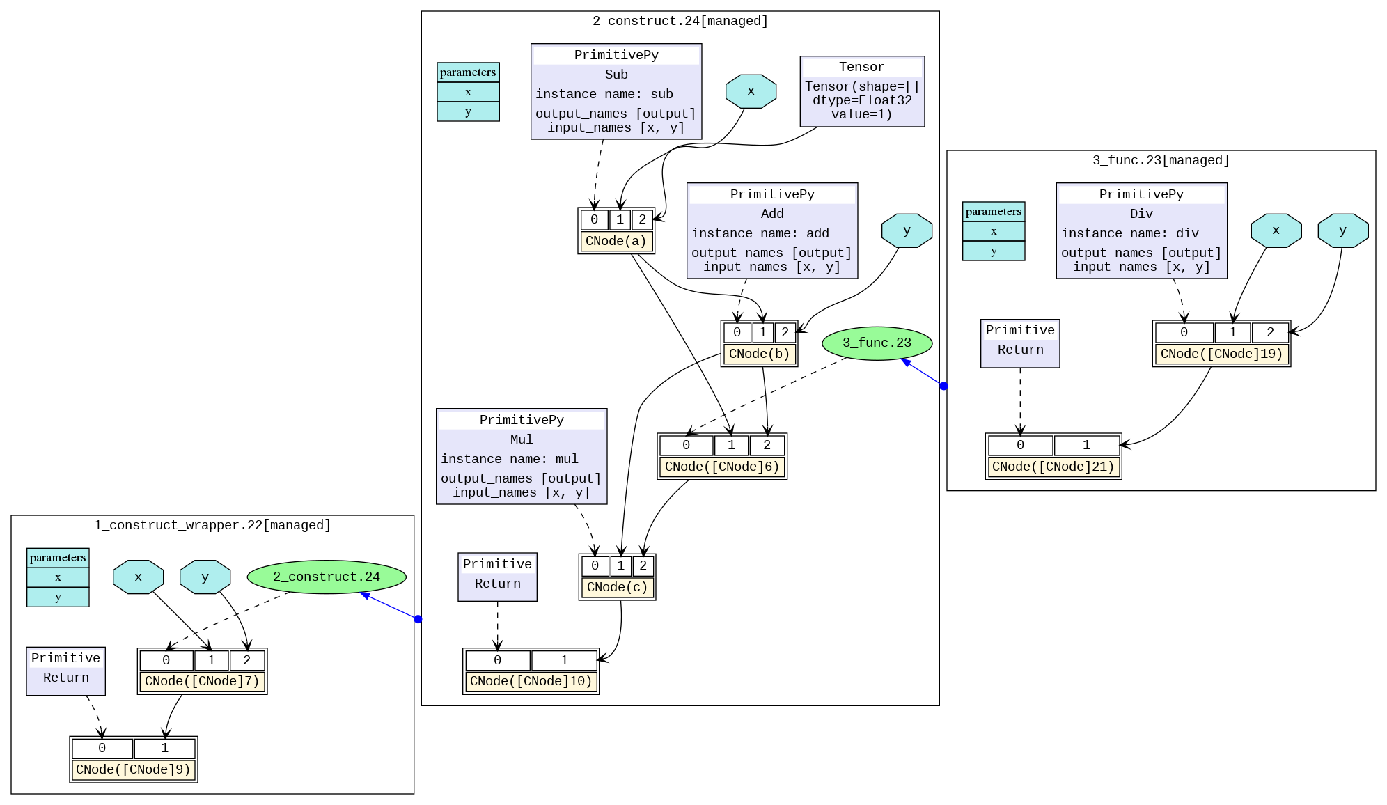
对于算子比较多的模型，图片会过于庞大，推荐使用可视化组件MindInsight对计算图进行可视化。

如何根据analyze_fail.dat文件分析图推导失败的原因

MindSpore在编译图的过程中，经常会出现abstract_specialize阶段的图推导失败的报错，通常我们能根据报错信息以及analyze_fail.dat文件，来定位出脚本中存在的问题。

例如执行下面一段代码：

import mindspore.context as context
import mindspore.nn as nn
from mindspore import Tensor
from mindspore.nn import Cell
from mindspore import ops
from mindspore import dtype as mstype
  7
context.set_context(mode=context.GRAPH_MODE)
context.set_context(save_graphs=True)
 10
class Net(nn.Cell):
   def __init__(self):
       super().__init__()
       self.add = ops.Add()
       self.sub = ops.Sub()
       self.mul = ops.Mul()
       self.div = ops.Div()
 18
   def func(x, y):
       return self.div(x, y)
 21
   def construct(self, x, y):
       a = self.sub(x, 1)
       b = self.add(a, y)
       c = self.mul(b, self.func(a, a, b))
       return c
 27
input1 = Tensor(3, mstype.float32)
input2 = Tensor(2, mstype.float32)
net = Net()
out = net(input1, input2)
print(out)

会出现如下的报错：

[EXCEPTION] ANALYZER(31946,7f6f03941740,python):2021-09-18-15:10:49.094.863 [mindspore/ccsrc/pipeline/jit/static_analysis/stack_frame.cc:85] DoJump] The parameters number of the function is 2, but the number of provided arguments is 3.
FunctionGraph ID : func.18
NodeInfo: In file test.py(19)
   def func(x, y):
  5
Traceback (most recent call last):
 File "test.py", line 31, in <module>
   out = net(input1, input2)
 File "/home/workspace/mindspore/mindspore/nn/cell.py", line 404, in __call__
   out = self.compile_and_run(*inputs)
 File "/home/workspace/mindspore/mindspore/nn/cell.py", line 682, in compile_and_run
   self.compile(*inputs)
 File "/home/workspace/mindspore/mindspore/nn/cell.py", line 669, in compile
   _cell_graph_executor.compile(self, *inputs, phase=self.phase, auto_parallel_mode=self._auto_parallel_mode)
 File "/home/workspace/mindspore/mindspore/common/api.py", line 542, in compile
   result = self._graph_executor.compile(obj, args_list, phase, use_vm, self.queue_name)
TypeError: mindspore/ccsrc/pipeline/jit/static_analysis/stack_frame.cc:85 DoJump] The parameters number of the function is 2, but the number of provided arguments is 3.
FunctionGraph ID : func.18
NodeInfo: In file test.py(19)
   def func(x, y):
 21
The function call stack (See file '/home/workspace/mindspore/rank_0/om/analyze_fail.dat' for more details):
# 0 In file test.py(26)
       return c
       ^
# 1 In file test.py(25)
       c = self.mul(b, self.func(a, a, b))
                       ^

以上的报错信息为：“TypeError: mindspore/ccsrc/pipeline/jit/static_analysis/stack_frame.cc:85 DoJump] The parameters number of the function is 2, but the number of provided arguments is 3…”。表明FunctionGraph ID : func.18只需要2个参数，但是却提供了3个参数。从“The function call stack …”中，可以知道出错的代码为：“In file test.py(25) … self.func(a, a, b)”，易知是该处的函数调用传入参数的数目过多。

但如果报错信息不直观或者需要查看IR中已推导出的部分图信息，我们使用文本编辑软件（例如，vi）打开报错信息中的提示的文件（第22行括号中）：/home/workspace/mindspore/rank_0/om/analyze_fail.dat，内容如下：

# [No.1] construct_wrapper.0
# In file test.py(22)/    def construct(self, x, y):/
funcgraph fg_0(
       %para1 : Tensor(F32)[]    # x
       , %para2 : Tensor(F32)[]    # y
   ) {
  7
#------------------------> 0
   %1 = FuncGraph::fg_3(%para1, %para2)    #(Tensor(F32)[], Tensor(F32)[])    # fg_3=construct.3 #scope: Default
     # In file test.py(26)/        return c/#[CNode]2
   Primitive::Return{prim_type=1}(%1)    #(Undefined) #scope: Default
     # In file test.py(26)/        return c/#[CNode]1
}
# order:
#   1: construct_wrapper.0:[CNode]2{[0]: ValueNode<FuncGraph> construct.3, [1]: x, [2]: y}
#   2: construct_wrapper.0:[CNode]1{[0]: ValueNode<Primitive> Return, [1]: [CNode]2}
 17
 18
# [No.2] construct.3
# In file test.py(22)/    def construct(self, x, y):/
funcgraph fg_3(
       %para3 : Tensor(F32)[]    # x
       , %para4 : Tensor(F32)[]    # y
   ) {
   %1 : Tensor(F32)[] = DoSignaturePrimitive::S-Prim-Sub{prim_type=1}[input_names=["x", "y"], output_names=["output"]](%para3, I64(1))    #(Tensor(F32)[], I64) #scope: Default
     # In file test.py(23)/        a = self.sub(x, 1)/#a
   %2 : Tensor(F32)[] = DoSignaturePrimitive::S-Prim-Add{prim_type=1}[input_names=["x", "y"], output_names=["output"]](%1, %para4)    #(Tensor(F32)[], Tensor(F32)[]) #scope: Default
     # In file test.py(24)/        b = self.add(a, y)/#b
 29
#------------------------> 1
   %3 = FuncGraph::fg_18(%1, %1, %2)    #(Tensor(F32)[], Tensor(F32)[], Tensor(F32)[])    # fg_18=func.18 #scope: Default
     # In file test.py(25)/        c = self.mul(b, self.func(a, a, b))/#[CNode]5
   %4 = DoSignaturePrimitive::S-Prim-Mul{prim_type=1}[input_names=["x", "y"], output_names=["output"]](%2, %3)    #(Tensor(F32)[], Undefined) #scope: Default
     # In file test.py(25)/        c = self.mul(b, self.func(a, a, b))/#c
   Primitive::Return{prim_type=1}(%4)    #(Undefined) #scope: Default
     # In file test.py(26)/        return c/#[CNode]4
}
# order:
#   1: construct.3:a{[0]: a, [1]: ValueNode<Int64Imm> 1, [2]: ValueNode<Float> Float32}
#   2: construct.3:a{[0]: ValueNode<DoSignaturePrimitive> S-Prim-Sub, [1]: x, [2]: ValueNode<Int64Imm> 1}
#   3: construct.3:b{[0]: ValueNode<DoSignaturePrimitive> S-Prim-Add, [1]: a, [2]: y}
#   4: construct.3:[CNode]5{[0]: ValueNode<FuncGraph> func.18, [1]: a, [2]: a, [3]: b}
#   5: construct.3:c{[0]: ValueNode<DoSignaturePrimitive> S-Prim-Mul, [1]: b, [2]: [CNode]5}
#   6: construct.3:[CNode]4{[0]: ValueNode<Primitive> Return, [1]: c}
 45
 46
#===============================================================================
# num of function graphs in stack: 2

analyze_fail.dat文件与前文介绍过的.dat文件格式一致，唯一有区别的地方在于analyze_fail.dat文件中会指出推导出错的节点所在的位置。我们不断搜索------------------------>并来到最后一处该箭头出现的位置，即第30行的------------------------> 1。该最后一处箭头指向了推导出错的节点，为%3 = FuncGraph::fg_18(%1, %1, %2) ...，表达了该节点在IR中的信息，如何查看dat文件前文dat文件介绍一节中已经介绍，此处不再赘述。根据(%1, %1, %2)可知，该节点的输入参数有三个。从源码解析调用栈中可以知道实际该函数为self.func，在脚本中的定义为def dunc(x, y):...。在函数定义中，只需要两个参数，故会在此处出现推导失败的报错，我们需要修改脚本中传入的参数个数以解决该问题。