AI Industrial Flow Simulation Model (DongFang YuFeng)
![]()
![]()
![]()
Introduction
DongFang·YuFeng built based on Ascend AI, is an efficient and high-accuracy AI simulation model for forecasting flow fields over airfoils of the airliner. With the support of MindSpore, the ability to simulate complex flows has been effectively improved. The simulation time is shortened to 1/24 of that in traditional Computational Fluid Dynamics (CFD) and the number of wind tunnel tests is reduced.Additionally, “DongFang·YuFeng” is capable of predicting the areas with sharp changes in the flow field accurately, and the averaged error of the whole flow field can be reduced to 1e-4 magnitude, reaching the industrial standard.

This tutorial will introduce the research background and technical path of “DongFang·YuFeng” and show how to use MindSpore Flow to realize the training and fast inference of the model, as well as visualized analysis of the flow field, so as to quickly obtain the physical information of the flow field.
Background
Civil aircraft aerodynamic design level directly determines the “four characteristics” of aircraft, namely safety, comfort, economy and environmental protection. Aerodynamic design of aircraft, as one of the most basic and core technologies in aircraft design, has different research needs and priorities in different stages of aircraft flight envelope (take-off, climb, cruise, descent, landing, etc.). For example, in the take-off phase, engineers will focus more on external noise and high lift-drag ratio, while in the cruise phase they will focus on fuel and energy efficiency. The flow simulation technology is widely used in aircraft aerodynamic design. Its main purpose is to obtain the flow field characteristics (velocity, pressure, etc.) of the simulation target through numerical methods, and then analyze the aerodynamic performance parameters of the aircraft, so as to achieve the optimization design of the aerodynamic performance of the aircraft.

Currently, the aerodynamic simulation of aircraft usually uses commercial simulation software to solve the governing equations and obtain the corresponding aerodynamic performance parameters (lift and drag, pressure, velocity, etc.). However, regardless of the CFD-based simulation software, the following steps are involved:
Physical modeling. The physical problems are abstracted and simplified to model the 2D/3D fluid and solid computational domain of the related geometry.
Mesh partition. The computing domain is divided into face/volume units of corresponding size to resolve turbulence in different areas and different scales.
Numerical discretization. The integral, differential and partial derivative terms in the governing equation are discretized into algebraic form through different order numerical formats to form corresponding algebraic equations.
Solution of governing equation. Use the numerical methods (such as
SIMPLE,PISOetc.) to solve the discrete governing equations iteratively, and calculate the numerical solutions at discrete time/space points.Post-processing. After the solution, use the flow field post-processing software to conduct qualitative and quantitative analysis and visualization of the simulation results and verify the accuracy of the results.

However, with the shortening of aircraft design and development cycle, the existing aerodynamic design methods have many limitations. Thus, in order to make the aerodynamic design level of airliner catch up with the two major aviation giants, Boeing and Airbus, it is necessary to develop advanced aerodynamic design means and combine advanced technologies such as artificial intelligence to establish fast aerodynamic design tools suitable for model design, thereby improving its simulation capability for complex flows and reducing the number of wind tunnel tests, as well as reducing design and research and development costs.

In the design of aircraft, the drag distribution of the wing is about 52% of the overall flight drag. Therefore, the wing shape design is very important for the whole flight performance of the aircraft. However, the high-fidelity CFD simulation of 3D wing requires millions of computational grids, which consumes a lot of computational resources and takes a long computational cycle. To improve the efficiency of simulation design, the design optimization of the two-dimensional section of the 3D wing is usually carried out first, and this process often requires repeated iterative CFD calculation for thousands of pairs of airfoils and their corresponding working conditions. Among these airfoils, the supercritical airfoil has an important application in high-speed cruise. Compared with the common airfoil, the supercritical airfoil has a fuller head, which reduces the peak negative pressure at the leading edge, and makes the airflow reach the sound velocity later, i.e. the critical Mach number is increased. At the same time, the middle of the upper surface of supercritical airfoil is relatively flat, which effectively controls the further acceleration of the upper airfoil airflow, reduces the intensity and influence range of the shock wave, and delays the shock-induced boundary layer separation on the upper surface. Therefore, supercritical airfoils with higher critical Mach numbers must be considered in wing shapes, since they can significantly improve aerodynamic performance in the transonic range, reduce drag and improve attitude controllability.

However, the aerodynamic design of two-dimensional supercritical airfoils needs to be simulated for different shapes and inflow parameters, and there are still a lot of iterative computations, which result in a long design cycle. Therefore, it is particularly important to use AI’s natural parallel inference capabilities to shorten the research and development cycle. Based on this, COMAC and Huawei jointly released the industry’s first AI industrial flow simulation model – “DongFang·YuFeng”, which can detect changes in the geometry and flow parameters (angle of attack/Mach number) of the supercritical airfoil. The high-efficiency and high-precision inference of airfoil flow field of airliner is realized, and the flow field around airfoil and lift drag are predicted quickly and accurately.
Technical difficulties
In order to realize high-efficiency and high-precision flow field prediction of supercritical airfoil by AI, the following technical difficulties need to be overcome:
Airfoil meshes are uneven and flow feature extraction is difficult. O-type or C-type meshes are often used for fluid simulation of 2D airfoil computing domain. As shown in the figure, a typical O-shaped mesh is divided. In order to accurately calculate the flow boundary layer, the near-wall surface of the airfoil is meshed, while the far-field mesh is relatively sparse. This non-standard grid data structure increases the difficulty of extracting flow features.


Flow characteristics change significantly when different aerodynamic parameters or airfoil shapes change. As shown in the figure, when the angle of attack of the airfoil changes, the flow field will change dramatically, especially when the angle of attack increases to a certain degree, shock wave phenomenon will occur: that is, there is obvious discontinuity in the flow field. The pressure, velocity and density of the fluid on the wavefront are obviously changed abruptly.

The flow field in the shock region changes dramatically, and it is difficult to predict. Because the existence of shock wave has a significant impact on the flow field nearby, the flow field before and after shock wave changes dramatically, and the flow field changes are complex, making it difficult for AI to predict. The location of shock wave directly affects the aerodynamic performance design and load distribution of airfoil. Therefore, accurate capture of shock signals is very important but challenging.
Technical Path
Aiming at the technical difficulties mentioned above, we designed an AI model-based technology roadmap to construct the end-to-end mapping of airfoil geometry and its corresponding flow fields under different flow states, which mainly includes the following core steps:
First, we design an efficient AI data conversion tool to realize feature extraction of complex boundary and non-standard data of airfoil flow field, as shown in the data preprocessing module. Firstly, the regularized AI tensor data is generated by the grid conversion program of curvilinear coordinate system, and then the geometric coding method is used to enhance the extraction of complex geometric boundary features.
Secondly, the neural network model is used to map the airfoil configuration and the physical parameters of the flow field under different flow states, as shown in Figure ViT-based encoder-decoder. The input of the model is airfoil geometry information and aerodynamic parameters generated after coordinate transformation. The output of the model is the physical information of the flow field, such as velocity and pressure.
Finally, the weights of the network are trained using the multilevel wavelet transform loss function. Perform further decomposition and learning on abrupt high-frequency signals in the flow field, so as to improve prediction accuracy of areas (such as shock waves) that change sharply in the flow field, as shown in a module corresponding to the loss function.

Preparation
Before practice, ensure that MindSpore and MindSpore Flow of the latest versions have been correctly installed. If not, you can run the following command:
MindSpore installation page Install MindSpore。
MindSpore Flow installation page Install MindSpore Flow。
“DongFang · YuFeng” MindSpore Flow Implementation
The implementation of “DongFang·YuFeng” MindSpore Flow consists of the following six steps:
Configure network and training parameters
Creating and Loading Datasets
Model building
Model training
Result visualization
Model inference
[1]:
import os
import time
import numpy as np

import mindspore.nn as nn
import mindspore.ops as ops
from mindspore import context
from mindspore import dtype as mstype

from mindspore import save_checkpoint, jit, data_sink
from mindspore import set_seed

from mindflow.common import get_warmup_cosine_annealing_lr
from mindflow.pde import SteadyFlowWithLoss
from mindflow.loss import WaveletTransformLoss
from mindflow.cell import ViT
from mindflow.utils import load_yaml_config
The following src pacakage can be downloaded in applications/data_driven/airfoil/2D_steady/src.
[2]:
from src import AirfoilDataset, calculate_eval_error, plot_u_and_cp, get_ckpt_summ_dir
set_seed(0)
np.random.seed(0)

context.set_context(mode=context.GRAPH_MODE,
                    save_graphs=False,
                    device_target="Ascend",
                    device_id=6)
use_ascend = context.get_context("device_target") == "Ascend"
Configure network and training parameters
Read four types of parameters from the configuration file, which are model-related parameters (model), data-related parameters (data), optimizer-related parameters (optimizer), output-related parameters (ckpt) and validation-related parameters(eval).You can get these parameters from config.
[4]:
config = load_yaml_config("config.yaml")
data_params = config["data"]
model_params = config["model"]
optimizer_params = config["optimizer"]
ckpt_params = config["ckpt"]
eval_params = config["eval"]
Creating and Loading Datasets
Download dataset link:data_driven/airfoil/2D_steady/dataset
The data is a mindrecord type file. The code for reading and viewing the data shape is as follows:
This file contains 2808 flow field data for 51 supercritical airfoils in the range of Ma=0.73 and different angles of attack (- 2.0 to 4.6). Where, the data dimensions of input are (13, 192, 384), 192, and 384 are the grid resolution after Jacobi conversion, and 13 are different feature dimensions, respectively (\(AOA\), \(x\), \(y\), \(x_{i,0}\), \(y_{i,0}\), \(\xi_x\), \(\xi_y\), \(\eta_x\), \(\eta_y\), \(x_\xi\), \(x_\eta\), \(y_\xi\), \(y_\eta\)).
The data dimension of Label is (288, 768), which can be passed through the patchify function in utils.py(16 × 16). The flow field data (u, v, p) obtained after the operation can be restored to (3, 192, 384) through the unpatchify operation in utils.py. Users can customize and select based on their own network input and output design.
First, convert the CFD dataset into tensor data, and then convert the tensor data into MindRecord. Design an AI data efficient conversion tool to achieve feature extraction of complex boundary and non-standard data of airfoil flow fields. The information of x, y, and u before and after conversion is shown in the following figure.

Currently, AI fluid simulation supports training using local datasets. You can use the MindDataset interface to configure dataset options. You need to specify the location of the MindRecord dataset file.
The default value of the train_size field in the config.yaml file is 0.8, indicating that the default ratio of the training set to the validation set is 4:1 in “train” mode. You can modify the value. The default value of finetune_size in the config.yaml file is 0.2, indicating that the default ratio of the training set to the validation set is 1:4 in “finetune” mode. You can modify the value. When the training mode is set to eval, all data sets are used as validation sets.
The min_value_list and min_value_list fields in the config.yaml file indicate the maximum and minimum values of the angle of attack, x information after geometric encoding, and y information after geometric encoding, respectively.
The “train_num_list” field and “test_num_list” field in the config.yaml file indicate the airfoil start number list corresponding to the training and validation data sets respectively. Each group of data contains 50 airfoil data. For example, if the value of the “train_num_list” field is [0], it indicates 50 pieces of airfoil data corresponding to the training set from 0 to 49.
[ ]:
mindrecord_name = "flowfiled_000_050.mind"
dataset = ds.MindDataset(dataset_files=mindrecord_name, shuffle=False)
dataset = dataset.project(["inputs", "labels"])
print("samples:", dataset.get_dataset_size())
for data in dataset.create_dict_iterator(num_epochs=1, output_numpy=False):
    input = data["inputs"]
    label = data["labels"]
    print(input.shape)
    print(label.shape)
    break
[ ]:
method = model_params['method']
batch_size = data_params['batch_size']
model_name = "_".join([model_params['name'], method, "bs", str(batch_size)])
ckpt_dir, summary_dir = get_ckpt_summ_dir(ckpt_params, model_name, method)
max_value_list = data_params['max_value_list']
min_value_list = data_params['min_value_list']
data_group_size = data_params['data_group_size']
dataset = AirfoilDataset(max_value_list, min_value_list, data_group_size)

train_list, eval_list = data_params['train_num_list'], data_params['test_num_list']
train_dataset, eval_dataset = dataset.create_dataset(data_params['data_path'],
                                                     train_list,
                                                     eval_list,
                                                     batch_size=batch_size,
                                                     shuffle=False,
                                                     mode="train",
                                                     train_size=data_params['train_size'],
                                                     finetune_size=data_params['finetune_size'],
                                                     drop_remainder=True)
model_name: ViT_exp_bs_32
summary_dir: ./summary_dir/summary_exp/ViT_exp_bs_32
ckpt_dir: ./summary_dir/summary_exp/ViT_exp_bs_32/ckpt_dir
total dataset : [0]
train dataset size: 2246
test dataset size: 562
train batch dataset size: 70
test batch dataset size: 17
Model Building
The following uses the ViT model as an example. The model is built through the ViT interface defined by the MindSpore Flow package. You need to specify the parameters of the ViT model. You can also build your own model.The most important parameters of the ViT model are the depth, embed_dim, and num_heads of the encoder and decoder, which respectively control the number of layers in the model, the length of the implicit vector, and the number of heads of the multi-head attention mechanism. The default values of the parameters are as follows:
[7]:
if use_ascend:
    compute_dtype = mstype.float16
else:
    compute_dtype = mstype.float32
model = ViT(in_channels=model_params[method]['input_dims'],
            out_channels=model_params['output_dims'],
            encoder_depths=model_params['encoder_depth'],
            encoder_embed_dim=model_params['encoder_embed_dim'],
            encoder_num_heads=model_params['encoder_num_heads'],
            decoder_depths=model_params['decoder_depth'],
            decoder_embed_dim=model_params['decoder_embed_dim'],
            decoder_num_heads=model_params['decoder_num_heads'],
            compute_dtype=compute_dtype
            )
Loss function and optimizer
In order to improve the prediction accuracy of the high and low frequency information of the convection field, especially the error of the shock region, a multi-stage wavelet transform function wave_loss is used as the loss function, where wave_level can determine the number of wavelet series to be used. It is suggested that two or three levels of wavelet transforms can be used. In the process of network training, we chose Adam optimizer.
[8]:
# prepare loss scaler
if use_ascend:
    from mindspore.amp import DynamicLossScaler, all_finite, init_status
    loss_scaler = DynamicLossScaler(1024, 2, 100)
else:
    loss_scaler = None
steps_per_epoch = train_dataset.get_dataset_size()
wave_loss = WaveletTransformLoss(wave_level=optimizer_params['wave_level'])
problem = SteadyFlowWithLoss(model, loss_fn=wave_loss)
# prepare optimizer
epochs = optimizer_params["epochs"]
lr = get_warmup_cosine_annealing_lr(lr_init=optimizer_params["lr"],
                                    last_epoch=epochs,
                                    steps_per_epoch=steps_per_epoch,
                                    warmup_epochs=1)
optimizer = nn.Adam(model.trainable_params() + wave_loss.trainable_params(), learning_rate=Tensor(lr))
Train function
With MindSpore>= 2.0.0, you can train neural networks using functional programming paradigms, and single-step training functions are decorated with jit. The data_sink function is used to transfer the step-by-step training function and training dataset.
[ ]:
def forward_fn(x, y):
    loss = problem.get_loss(x, y)
    if use_ascend:
        loss = loss_scaler.scale(loss)
    return loss

grad_fn = ops.value_and_grad(forward_fn, None, optimizer.parameters, has_aux=False)

@jit
def train_step(x, y):
    loss, grads = grad_fn(x, y)
    if use_ascend:
        status = init_status()
        loss = loss_scaler.unscale(loss)
        if all_finite(grads, status):
            grads = loss_scaler.unscale(grads)
    loss = ops.depend(loss, optimizer(grads))
    return loss

train_sink_process = data_sink(train_step, train_dataset, sink_size=1)

Model training
During model training, inference is performed during model training. You can directly load the test data set and output the inference precision in the test set after n epochs are trained.
[ ]:
print(f'pid: {os.getpid()}')
print(f'use_ascend : {use_ascend}')
print(f'device_id: {context.get_context("device_id")}')

eval_interval = eval_params['eval_interval']
plot_interval = eval_params['plot_interval']
save_ckt_interval = ckpt_params['save_ckpt_interval']
# train process
for epoch in range(1, 1+epochs):
    # train
    time_beg = time.time()
    model.set_train(True)
    for step in range(steps_per_epoch):
        step_train_loss = train_sink_process()
    print(f"epoch: {epoch} train loss: {step_train_loss} epoch time: {time.time() - time_beg:.2f}s")
    # eval
    model.set_train(False)
    if epoch % eval_interval == 0:
        calculate_eval_error(eval_dataset, model)
    if epoch % plot_interval == 0:
        plot_u_and_cp(eval_dataset=eval_dataset, model=model,
                      grid_path=data_params['grid_path'], save_dir=summary_dir)
    if epoch % save_ckt_interval == 0:
        ckpt_name = f"epoch_{epoch}.ckpt"
        save_checkpoint(model, os.path.join(ckpt_dir, ckpt_name))
        print(f'{ckpt_name} save success')
pid: 71126
use_ascend : True
device_id: 6
total dataset : [0]
train dataset size: 2246
test dataset size: 562
train batch dataset size: 70
test batch dataset size: 17
model_name: ViT_exp_bs_32
summary_dir: ./summary_dir/summary_exp/ViT_exp_bs_32
ckpt_dir: ./summary_dir/summary_exp/ViT_exp_bs_32/ckpt_dir
epoch: 1 train loss: 2.855625 time cost: 99.03s
epoch: 2 train loss: 2.7128317 time cost: 11.67s
epoch: 3 train loss: 2.5762033 time cost: 11.34s
epoch: 4 train loss: 2.4458356 time cost: 11.62s
epoch: 5 train loss: 2.3183048 time cost: 11.35s
...
epoch: 996 train loss: 0.07591154 time cost: 10.27s
epoch: 997 train loss: 0.07530779 time cost: 10.57s
epoch: 998 train loss: 0.07673213 time cost: 11.10s
epoch: 999 train loss: 0.07614599 time cost: 10.56s
epoch: 1000 train loss: 0.07557951 time cost: 10.25s
================================Start Evaluation================================
mean l1_error : 0.00028770750813076604, max l1_error : 0.09031612426042557, average l1_error : 0.015741700749512186, min l1_error : 0.002440142212435603, median l1_error : 0.010396258905529976
mean u_error : 0.0003678269739098409, max u_error : 0.1409306526184082, average u_error : 0.02444652929518591, min u_error : 0.002988457679748535, median u_error : 0.018000304698944092
mean v_error : 0.0001693408951670041, max v_error : 0.025479860603809357, average v_error : 0.0065298188753384985, min v_error : 0.0011983513832092285, median v_error : 0.005558336153626442
mean p_error : 0.0003259546544594581, max p_error : 0.11215704679489136, average p_error : 0.016248753842185524, min p_error : 0.0014863014221191406, median p_error : 0.009315729141235352
mean Cp_error : 0.0004100774693891735, max Cp_error : 0.052939414978027344, average Cp_error : 0.00430003712501596, min Cp_error : 0.0008158683776855469, median Cp_error : 0.0018098950386047363
=================================End Evaluation=================================
predict total time: 27.737457513809204 s
================================Start Plotting================================
./summary_dir/summary_exp/ViT_exp_bs_32/U_and_Cp_compare.png
================================End Plotting================================
Plot total time: 27.499852657318115 s
Train epoch time: 122863.384 ms, per step time: 1755.191 ms
epoch_1000.ckpt save success
Result visualization
Surface pressure distribution, flow field distribution and error statistics predicted by AI and CFD when airfoil geometry changes.

Surface pressure distribution, flow field distribution and error statistics predicted by AI and CFD when the angle of attack changes.

Surface pressure distribution, flow field distribution and error statistics predicted by AI and CFD when incoming flow Mach number changes.

Model inference
After model training is complete, you can call the train function in train.py. If train_mode is set to “eval”, inference can be performed. If train_mode is set to “finetune”, transfer learning can be performed.
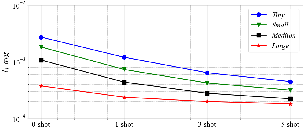
When designing a new airfoil, various initial boundary conditions (such as different angles of attack or Mach number) need to be considered for aerodynamic performance evaluation. In order to improve the generalization of the model and improve its utility in engineering scenarios, we can adopt the transfer learning mode. The method is as follows: pre-training the model in large-scale datasets, and fine-tuning the model in small datasets, so as to realize the inference generalization of the model to the new working conditions. Considering the trade-off between precision and time consumption, we considered four different size datasets to obtain different pre-trained models. Compared with pre-training on smaller datasets, pre-training requires less time, but the prediction precision is lower. Pre-training on larger data sets can produce more accurate results, but requires more pre-training time.
The results of the transfer learning are shown in the following figure. When the model is pre-trained using tiny data sets, at least three new flow fields are required to achieve 4e-4 accuracy. In contrast, when the model is pre-trained using small, medium, or large data sets, only a new flow field is required and an accuracy of 1e-4 can be maintained. In addition, \(l_{1\_avg}\) can be reduced by at least 50% by transfer learning using five flow fields. The pre-trained model with large data sets can predict the flow field with high precision in the case of zero-shot. The fine-tuning results obtained using datasets of different sizes and sizes are shown in the figure below. The fine-tuning takes much less time than the sample generation, and when the fine-tuning is complete, other operating conditions of the new airfoil can be quickly reasoned. Therefore, the fine-tuning technology based on transfer learning is of great value in engineering application.