Functional and Object-Oriented Fusion Programming Paradigm
![]()
Programming paradigm refers to the programming style or programming approach of a programming language. Typically, AI frameworks rely on the programming paradigm of the programming language used by the front-end programming interface for the construction and training of neural networks. MindSpore, as an AI+scientific computing convergence computing framework, provides object-oriented programming and functional programming support for AI and scientific computing scenarios, respectively. At the same time, in order to enhance the flexibility and ease of use of the framework, a functional + object-oriented fusion programming paradigm is proposed, which effectively reflects the advantages of functional automatic differentiation mechanism.
The following describes each of the three types of programming paradigms supported by MindSpore and their simple examples.
Object-oriented Programming
Object-oriented programming (OOP) is a programming method that decomposes programs into modules (classes) that encapsulate data and related operations, with objects being instances of classes. Object-oriented programming uses objects as the basic unit of a program, encapsulating the program and data in order to improve the reusability, flexibility and extensibility of the software, and the program in the object can access and often modify the data associated with the object.
In a general programming scenario, code and data are the two core components. Object-oriented programming is to design data structures for specific objects to define classes. The class usually consists of the following two parts, corresponding to code and data, respectively:
Methods
Attributes
For different objects obtained after the instantiation of the same Class, the methods and attributes are the same, but the difference is the values of the attributes. The different attribute values determine the internal state of the object, so OOP can be good for state management.
The following is an example of a simple class constructed in Python:
class Sample: #class declaration
    def __init__(self, name): # class constructor (code)
        self.name = name # attribute (data)

    def set_name(self, name): # method declaration (code)
        self.name = name # method implementation (code)
For constructing a neural network, the primary component is the network layer (Layer), and a neural network layer contains the following components:
Tensor Operation
Weights
These two correspond exactly to the Methods and Attributes of the class, and the weights themselves are the internal states of the neural network layer, so using the class to construct Layers naturally fits its definition. In addition, we wish to use the neural network layer for stacking and construct deep neural networks when programming, and new Layer classes can be easily constructed by combining Layer objects using OOP programming. In addition, we wish to use neural network layers for stacking and constructing deep neural networks when programming, and new Layer classes can be easily constructed by combining Layer objects by using OOP programming.
The following is an example of a neural network class constructed by using MindSpore:
from mindspore import nn, Parameter
from mindspore.common.initializer import initializer

class Linear(nn.Cell):
    def __init__(self, in_features, out_features, has_bias): # class constructor (code)
        super().__init__()
        self.weight = Parameter(initializer('normal', [out_features, in_features], mindspore.float32), 'weight') # layer weight (data)
        self.bias = Parameter(initializer('zeros', [out_features], mindspore.float32), 'bias') # layer weight (data)

    def construct(self, inputs): # method declaration (code)
        output = ops.matmul(inputs, self.weight.transpose(0, 1)) # tensor transformation (code)
        output = output + self.bias # tensor transformation (code)
        return output
In addition to the construction of the neural network layer by using the object-oriented programming paradigm, MindSpore supports pure object-oriented programming to construct the neural network training logic, where the forward computation, back propagation, gradient optimization and other operations of the neural network are constructed by using classes. The following is an example of pure object-oriented programming.
import mindspore
import mindspore.nn as nn
from mindspore import value_and_grad

class TrainOneStepCell(nn.Cell):
    def __init__(self, network, optimizer):
        super().__init__()
        self.network = network
        self.optimizer = optimizer
        self.grad_fn = value_and_grad(self.network, None, self.optimizer.parameters)

    def construct(self, *inputs):
        loss, grads = self.grad_fn(*inputs)
        self.optimizer(grads)
        return loss

network = nn.Dense(5, 3)
loss_fn = nn.BCEWithLogitsLoss()
network_with_loss = nn.WithLossCell(network, loss_fn)
optimizer = nn.SGD(network.trainable_params(), 0.001)
trainer = TrainOneStepCell(network_with_loss, optimizer)
At this point, both the neural network and its training process are managed by using classes that inherit from nn.Cell, which can be easily compiled and accelerated as a computational graph.
Functional Programming
Functional programming is a programming paradigm that treats computer operations as functions and avoids the use of program state and mutable objects.
In the functional programming, functions are treated as first-class citizens, which means they can be bound to names (including local identifiers), passed as arguments, and returned from other functions, just like any other data type. This allows programs to be written in a declarative and composable style, where small functions are combined in a modular fashion. Functional programming is sometimes seen as synonymous with pure functional programming, a subset of functional programming that treats all functions as deterministic mathematical functions or pure functions. When a pure function is called with some given parameters, it will always return the same result and is not affected by any mutable state or other side effects.
The functional programming has two core features that make it well suited to the needs of scientific computing:
The programming function semantics are exactly equivalent to the mathematical function semantics.
Determinism, if the same input is given, the same output is returned. No side effects.
Due to this feature of determinism, by limiting side effects, programs can have fewer errors, are easier to debug and test, and are more suitable for formal verification.
MindSpore provides pure functional programming support. With the numerical computation interfaces provided by mindspore.numpy and mindspore.scipy, you can easily program scientific computations. The following is an example of using functional programming:
import mindspore.numpy as mnp
from mindspore import grad

grad_tanh = grad(mnp.tanh)
print(grad_tanh(2.0))
# 0.070650816

print(grad(grad(mnp.tanh))(2.0))
print(grad(grad(grad(mnp.tanh)))(2.0))
# -0.13621868
# 0.25265405
In line with the needs of the functional programming paradigm, MindSpore provides a variety of functional transformation interfaces, including automatic differentiation, automatic vectorization, automatic parallelism, just-in-time compilation, data sinking and other functional modules, which are briefly described below:
Automatic differentiation:
grad,value_and_grad, providing differential function transformation.Automatic vectorization: A higher-order function for mapping a function fn along the parameter axis.
Automatic parallelism:
shard, a functional operator slice, specifying the distribution strategy of the function input/output Tensor.Just-in-time compilation:
jit, which compiles a Python function into a callable MindSpore graph.Data sinking:
data_sink, transform the input function to obtain a function that can use the data sink pattern.
Based on the above function transformation interfaces, function transformations can be used quickly and efficiently to implement complex functions when using the functional programming paradigm.
Functional Differential Programming
Automatic Differentiation
Modern AI algorithm, such as deep learning, uses a large amount of data to learn and fit an optimized model with parameters. This training process often uses loss back-propagation to update parameters. Automatic differentiation (AD) is one of the key techniques.
Automatic differentiation is a derivation method between neumerical differentiation and symbolic differentiation. The key concept of AD is to divide the calculation of the computer program into a finite set with basic operations. The derivations of all the basic operations are known. After calculating the derivation of all the basic operations, AD uses chain rule to combine them and gets the final gradient.
The formula of chain rule is:
Based on how to connect the gradient of basic components, AD can be divided into forward mode AD and reverse mode AD.
Forward Automatic Differentiation (also known as tangent linear mode AD) or forward cumulative gradient (forward mode).
Reverse Automatic Differentiation (also known as adjoint mode AD) or reverse cumulative gradient (reverse mode).
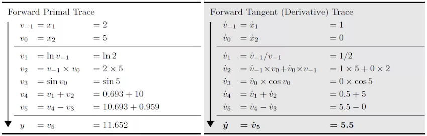
Let’s take formula (2) as an example to introduce the specific calculation method of forward and reverse differentiation:
When we use the forward automatic differentiation formula (2) at \(x_{1}=2, x_{2}=5\), \(frac{partial y}{partial x_{1}}\), the direction of derivation of forward automatic differentiation is consistent with the evaluation direction of the original function, and the original function result and the differential result can be obtained at the same time.
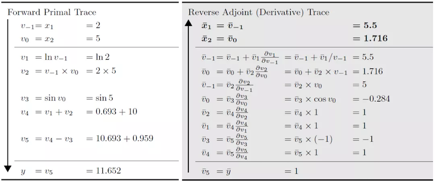
When using reverse automatic differentiation, the direction of differentiation of the reverse automatic differentiation is opposite to the evaluation direction of the original function, and the differential result depends on the running result of the original function.
MindSpore first developed automatic differentiation based on the reverse pattern, and implemented forward differentiation on the basis of this method.
In order to explain the differences between forward mode AD and reverse mode AD in further, we generalize the derived function to F, which has an N input and an M output:
The gradient of function \(F()\) is a Jacobian matrix.
Forward Mode AD
In forward mode AD, the calculation of gradient starts from inputs. So, for each calculation, we can get the gradient of outputs with respect to one input, which is one column of the Jacobian matrix.
In order to get this value, AD divies the program into a series of basic operations. The gradient rules of these basic operations is known. The basic operation can also be represented as a function \(f\) with \(n\) inputs and \(m\) outputs:
Since we have defined the gradient rule of \(f\), we know the jacobian matrix of \(f\). So we can calculate the Jacobian-vector-product (Jvp) and use the chain rule to get the gradient outoput.
Reverse Mode AD
In reverse mode AD, the calculation of gradient starts from outputs. So, for each calculation, we can get the gradient of one output with respect to inputs, which is one row of the Jacobian matrix.
In order to get this value, AD divies the program into a series of basic operations. The gradient rules of these basic operations is known. The basic operation can also be represented as a function \(f\) with n inputs and m outputs:
Since we have defined the gradient rule of \(f\), we know the jacobian matrix of \(f\). So we can calculate the Vector-Jacobian-product (Vjp) and use the chain rule to get the gradient outoput.
grad Implementation
grad uses reverse mode AD, which calcultes gradients from network outputs.
grad Design
Consuming that the origin function of defining model is as follows:
Then the gradient of \(f()\) to \(x\) is:
The formula of \(\frac{df}{dy}\) and \(\frac{df}{dz}\) is similar to \(\frac{df}{dx}\).
Based on chain rule, we define gradient function bprop: dout->(df, dinputs) for every functions (including operators and graph). Here, df means gradients with respect to free variables (variables defined outside the function) and dinputs is gradients to function inputs. Then we use total derivative rule to accumulate (df, dinputs) to correspond variables.
MindIR has developed the formulas for branching, loops and closures. So if we define the gradient rules correctly, we can get the correct gradient.
Define operator K, backward mode AD can be represented as:
v = (func, inputs)
F(v): {
    (result, bprop) = K(func)(K(inputs))
    df, dinputs = bprop(dout)
    v.df += df
    v.dinputs += dinputs
}
grad Algorithm Implementation
In grad process, the function that needs to calculate gradient will be taken out and used as the input of automatic differentiation module.
AD module will map input function to gradient fprop.
The output gradient has form fprop = (forward_result, bprop). forward_result is the output node of the origin function. bprop is the gradient function which relies on the closure object of fprop. bprop has only one input dout. inputs and outputs are the called inputs and outputs of fprop.
  MapObject(); // Map ValueNode/Parameter/FuncGraph/Primitive object
  MapMorphism(); // Map CNode morphism
  res = k_graph(); // res is fprop object of gradient function
When generating gradient function object, we need to do a series of mapping from origin function to gradient function. These mapping will generate gradient function nodes and we will connect these nodes according to reverse mode AD rules.
For each subgraph of origin function, we will create an DFunctor object, for mapping the original function object to a gradient function object. Dfunctor will run MapObject and MapMorphism to do the mapping.
MapObject implements the mapping of the original function node to the gradient function node, including the mapping of free variables, parameter nodes, and ValueNode.
MapFvObject(); // map free variables
MapParamObject(); // map parameters
MapValueObject(); // map ValueNodes
MapFvObjectmaps free variables.MapParamObjectmaps parameter nodes.MapValueObjectmainly mapsPrimitiveandFuncGraphobjects.
For FuncGraph, we need to create another DFunctor object and perform the mapping, which is a recursion process. Primitive defines the type of the operator. We need to define gradient function for every Primitive.
MindSpore defines these gradient functions in Python, taking sin operator for example:
import mindspore.ops as ops
from mindspore.ops._grad.grad_base import bprop_getters

@bprop_getters.register(ops.Sin)
def get_bprop_sin(self):
    """Grad definition for `Sin` operation."""
    cos = ops.Cos()

    def bprop(x, out, dout):
        dx = dout * cos(x)
        return (dx,)

    return bprop
x is the input to the original function object sin. out is the output of the original function object sin, and dout is the gradient input of the current accumulation.
When MapObject completes the mapping of the above nodes, MapMorphism recursively implements the state injection of CNode from the output node of the original function, establishes a backpropagation link between nodes, and realizes gradient accumulation.
grad Example
Let’s build a simple network to represent the formula:
And derive the input x of formula (13):
The structure of the network in formula (13) in MindSpore is implemented as follows:
import mindspore.nn as nn

class Net(nn.Cell):
    def __init__(self):
        super(Net, self).__init__()
        self.sin = ops.Sin()
        self.cos = ops.Cos()

    def construct(self, x):
        a = self.sin(x)
        out = self.cos(a)
        return out
The structure of a forward network is:

After the network is reversely differential, the resulting differential network structure is:

Forward Automatic Differentiation Implementation
Besides grad, Mindspore has developed forward mode automatic differentiation method jvp (Jacobian-Vector-Product).
Compared to reverse mode AD, forward mode AD is more suitable for networks whose input dimension is smaller than output dimension. Mindspore forward mode AD is developed based on reversed mode Grad function.

The network in black is the origin function. After the first derivative based on one input \(x\), we get the network in blue. The second is the blue plot for the \(v\) derivative, resulting in a yellow plot.
This yellow network is the forward mode AD gradient network of black network. Since blue network is a linear network for vector \(v\), there will be no connection between blue network and yellow network. So, all the nodes in blue are dangling nodes. We can use only blue and yellow nodes to calculate the gradient.
References
[1] Baydin, A.G. et al., 2018. Automatic differentiation in machine learning: A survey. arXiv.org. [Accessed September 1, 2021].
Functional + Object-Oriented Fusion Programming
Taking into account the flexibility and ease of use of the neural network model construction and training process, combined with MindSpore’s own functional automatic differentiation mechanism, MindSpore has designed a functional + object-oriented fusion programming paradigm for AI model training, which can combine the advantages of object-oriented programming and functional programming. The same set of automatic differentiation mechanism is also used to achieve the compatibility of deep learning back propagation and scientific computing automatic differentiation, supporting the compatibility of AI and scientific computing modeling from the bottom. The following is a typical process for the functional + object-oriented fusion programming:
Constructing neural networks with classes.
Instantiating neural network objects.
Constructing the forward function, and connecting the neural network and the loss function.
Using function transformations to obtain gradient calculation (back propagation) functions.
Constructing training process functions.
Calling functions for training.
The following is a simple example of functional + object-oriented fusion programming:
# Class definition
class Net(nn.Cell):
    def __init__(self):
        ......
    def construct(self, inputs):
        ......

# Object instantiation
net = Net() # network
loss_fn = nn.CrossEntropyLoss() # loss function
optimizer = nn.Adam(net.trainable_params(), lr) # optimizer

# define forward function
def forword_fn(inputs, targets):
    logits = net(inputs)
    loss = loss_fn(logits, targets)
    return loss, logits

# get grad function
grad_fn = value_and_grad(forward_fn, None, optim.parameters, has_aux=True)

# define train step function
def train_step(inputs, targets):
    (loss, logits), grads = grad_fn(inputs, targets) # get values and gradients
    optimizer(grads) # update gradient
    return loss, logits

for i in range(epochs):
    for inputs, targets in dataset():
        loss = train_step(inputs, targets)
As in the above example, object-oriented programming is used in the construction of the neural network, and the neural network layers are constructed in a manner consistent with the conventions of AI programming. When performing forward computation and backward propagation, MindSpore uses functional programming to construct the forward computation as a function, then obtains grad_fn by function transformation, and finally obtains the gradient corresponding to the weights by executing grad_fn.
The functional + object-oriented fusion programming ensures the ease of use of neural network construction and improves the flexibility of training processes such as forward computation and backward propagation, which is the default programming paradigm recommended by MindSpore.