Sharding Propagation

Background

Distributed operator, Tensor Layout, and Tensor Redistribution are fundamental concepts in op-level parallelism of MindSpore. In here, these concepts are introduced by examples. Here, we formally define them.

In op-level parallelism, we conduct SPMD (Single Program Multiple Data) style parallelism, that is, a single program is produced for all partitions. MindSpore transforms a stand-alone program to a parallel one. The transformation is fine-grained in the sense that each operator in the stand-alone program is substituted by (a) distributed operator(s), guaranteeing that the substitution is mathematically equivalent.

Distributed Operator

Distributed Operator: together, the distributed operators running on multiple devices preserve the same semantics of the stand-alone counterpart. That is, given the same input, the distributed operators’ output is the same as the stand-alone counterpart.

Say a matrix multiplication (MatMul) operator with two matrix X and W as input: Y = MatMul(X, W) is to be parallelized on 4 devices. If matrix X has copies on 4 devices, and W is split into 4 copies by column, one for each device, then the distributed operator corresponding to the stand-alone version of the MatMul operator is also MatMul, that is, MatMul operator is executed on each device. If X is split into 4 parts according to the column, W is cut into 4 parts by row, and each device gets a shard of X and W, then the distributed operator corresponding to the stand-alone version of the MatMul operator is MatMul->AllReduce, that is, the two operators of MatMul and AllReduce will be executed sequentially on each device to ensure mathematical equivalence.

Besides the SP (Single Program) part, MD (Multiple Data) part also needs to be specified. Before that, we first define the Sharding Strategy.

Sharding Strategy

Sharding Strategy: a Sharding Strategy for an operator is a two-dimensional array, specifying how many partitions to split each dimension of each input tensor for the operator.

From the sharding strategy, you can derive the Tensor Layout to describe how tensors are distributed across devices.

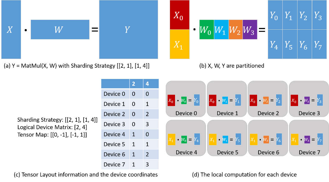
Tensor Layout

Tensor Layout: given a Sharding Strategy for an operator, the Tensor Layout is inferred to describe the distributions of the input tensors of the operator, which includes the Logical Device Matrix and the Tensor Map. The Logical Device Matrix is an one-dimensional array, describing how devices are arranged for the operator. The Tensor Map the dimensions of input tensors to dimensions of the device matrix, indicating that input tensors are partitioned across the Logical Device Matrix.

Use again the MatMul operator Y = MatMul(X, W). We configure the operator with Sharding Strategy [[2, 1], [1, 4]] and the corresponding Tensor Layout information is demonstrated in the following figure. X is partitioned into 2 parts along the row dimension, and W is partitioned into 4 parts along the column dimension (figure (b)). From the Sharding Strategy, the Logical Device Matrix and the Tensor Map are inferred, as shown in figure (c). The coordinates are also determined to describe the locations of devices in the Logical Device Matrix, based on which the distributions of tensors are determined. From the ‘2’ column in the coordinate table, Device 0—3 are assigned X₀, while Device 4—7 are assigned X₁. From the ‘4’ column in the coordinate table, Device 0 and Device 4 are assigned W₀, Device 1 and Device 5 are assigned W₁, Device 2 and Device 6 are assigned W₂, and Device 3 and Device 7 are assigned W₃. As a result, the local computation is determined, as shown in figure (d).

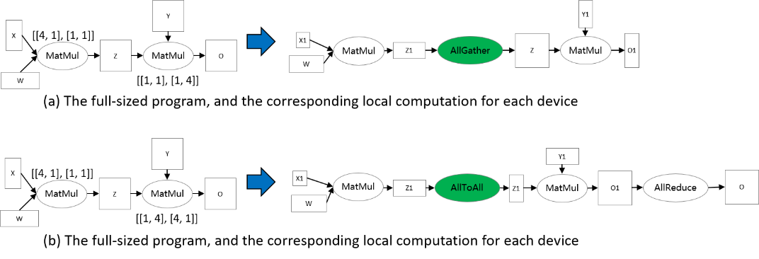
For two consecutive operators that are dependent, the Tensor Layouts defined by two operators may be inconsistent, due to either Logical Device Matrix or Tensor Map. We propose an algorithm, called Tensor Redistribution, that transforms the inconsistent Tensor Layout. We omit the algorithm here, and only give a definition.

Tensor Redistribution

Tensor Redistribution: given two inconsistent Tensor Layouts of a tensor, Tensor Redistribution is an algorithm that can transform from the source Tensor Layout to the target Tensor Layout, with minimum communication cost.

Here, the communication cost is measured by the bytes that each device transmits.

Say a two-operator example: Z = MatMul(X, W), O = MatMul(Z, Y). To make Tensor Redistribution effective, two operators are configured Sharding Strategies so that the Tensor Layouts of Z are inconsistent, as shown in the following figure. In figure (a), the output of the first MatMul is row partitioned, while the second MatMul requires that Z are full-sized. Therefore, an AllGather is inferred by Tensor Redistribution to perform the transformation[1]. In figure (b), the output tensor Z of the first matrix multiplication operator is row-sliced, while the second matrix multiplicator requires that the tensor Z be split by columns, so the tensor redistribution derivation needs to be inserted here to complete the conversion.

Sharding Propagation

Given a computation graph, Sharding Propagation is a functionality that propagates the Sharding Strategies from configured operator to the whole graph, with the goal of minimizing the communication cost in Tensor Redistribution.

The input of Sharding Propagation is a computation graph, in which nodes represent operators, and edges encode the data-dependency relationship of operators. From a model definition with some operators configured Sharding Strategies, Sharding Propagation executes as follows:

1. Generate possible Sharding Strategies for non-configured operators;

2. Generate Tensor Redistributions and the associated communication costs for each edge;

3. Start from the configured operators, and propagate the Sharding Strategies to non-configured operators using BFS, with the goal of minimizing the communication cost along each edge.

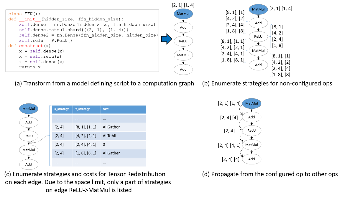
The following figure illustrates an example process of applying Sharding Propagation. Given an computation graph with some configured strategies, it first enumerates possible strategies for non-configured operators, as shown in figure (b). Next, it enumerates possible strategies and the Tensor Redistribution costs for each edge. Demonstrated in figure (c), the strategy for an edge is defined as a pair [s_strategy, t_strategy], where s_strategy and t_strategy denote Sharding Strategy for source operator and target operator, respectively. Finally, starting from the configured operator, it determines the next operator’s Sharding Strategy, such that the communication cost in Tensor Redistribution is minimized. The propagation ends when the Sharding Strategies for all operators are settled, as shown in figure (d).

How to use Sharding Propagation in MindSpore

Sample Code Description

Download the complete sample code:

https://gitee.com/mindspore/docs/tree/r2.0/docs/sample_code/sharding_propagation.

The directory structure is as follows, where rank_table_8pcs.json is the IP configuration for Ascend devices (see here for the explanation), train.py is the model definition, and run.sh is the execution script.

└─sample_code
    ├─sharding_propagatinon
    │      rank_table_8pcs.json
    │      run.sh
    │      train.py
    ...

Model definition

We use the FeedForward Network (FFN) as an example.

class FFN(Cell):
    def __init__(self):
        super().__init__()
        self.dense1 = Dense(64, 64)
        self.relu = ops.ReLU()
        self.dense2= Dense(64, 64)

    def construct(self, x):
        x = self.dense1(x)
        x = self.relu(x)
        x = self.dense2(x)
        return x

Configuring the Sharding Propagation

Annotate Sharding Strategy for a MatMul operator in FFN:

self.dense1.matmul.shard(((2, 1), (1, 4)))

Configure the search_mode as sharding_propagation in Auto_Parallel mode:

set_auto_parallel_context(parallel_mode="auto_parallel", search_mode="sharding_propagation")

Training the Model and Checking the Sharding Strategies

Run the command bash run.sh 8. By setting the context: save_graphs=2, the IR graphs in the compilation process are saved. We choose the IRs corresponding to device 0.

In step_parallel_begin_xxx.ir, each computation operator is annotated with a Sharding Strategy:

...
  %3(x) = MatMul(%1, %2) {instance name: matmul} primitive_attrs: {input_names: [x1, x2], out_strategy: None, transpose_x2: false, transpose_b: false, in_strategy: ((2, 1), (1, 4)), output_names: [output], transpose_a: false, transpose_x1: false}
 {in_strategy: ((2, 1), (1, 4))}      : (<Tensor[Float32], (64, 64)>, <Tensor[Float32], (64, 64)>) -> (<Tensor[Float32], (64, 64)>)
  %4([CNode]453) = Load($(@1_construct_wrapper.298:para4_dense1.bias), %para15_u)
      : (<Ref[Tensor(F32)], (64)>, <UMonad>) -> (<Tensor[Float32], (64)>)
  %5(x) = Add(%3, %4) {instance name: add} primitive_attrs: {output_names: [output], input_names: [x, y]}
 {in_strategy: ((2, 4), (4))}      : (<Tensor[Float32], (64, 64)>, <Tensor[Float32], (64)>) -> (<Tensor[Float32], (64, 64)>)
  %6(x) = ReLU(%5) {instance name: relu} primitive_attrs: {output_names: [output], input_names: [x]}
 {in_strategy: ((2, 4))}      : (<Tensor[Float32], (64, 64)>) -> (<Tensor[Float32], (64, 64)>)
  %7([CNode]447) = Load($(@1_construct_wrapper.298:para5_dense2.weight), %para15_u)
      : (<Ref[Tensor(F32)], (64, 64)>, <UMonad>) -> (<Tensor[Float32], (64, 64)>)
  %8(x) = MatMul(%6, %7) {instance name: matmul} primitive_attrs: {output_names: [output], transpose_a: false, input_names: [x1, x2], transpose_x2: false, transpose_x1: false, transpose_b: false}
 {in_strategy: ((2, 4), (4, 1))}      : (<Tensor[Float32], (64, 64)>, <Tensor[Float32], (64, 64)>) -> (<Tensor[Float32], (64, 64)>)
  %9([CNode]449) = Load($(@1_construct_wrapper.298:para6_dense2.bias), %para15_u)
      : (<Ref[Tensor(F32)], (64)>, <UMonad>) -> (<Tensor[Float32], (64)>)
  %10(x) = Add(%8, %9) {instance name: add} primitive_attrs: {output_names: [output], input_names: [x, y]}
 {in_strategy: ((2, 4), (4))}      : (<Tensor[Float32], (64, 64)>, <Tensor[Float32], (64)>) -> (<Tensor[Float32], (64, 64)>)
...

In xx_validate_xxx.ir, each input and output tensor in the computation operator is sliced according to the Sharding Strategy.

…
  %2(equivx) = MatMul(%0, %1) {instance name: matmul} primitive_attrs: {input_names: [x1, x2], out_strategy: None, transpose_x2: false, transpose_b: false, in_strategy: ((2, 1), (1, 4)), output_names: [output], transpose_a: false, transpose_x1: false}
 {in_strategy: ((2, 1), (1, 4))}      : (<Tensor[Float32], (32, 64)>, <Tensor[Float32], (64, 16)>) -> (<Tensor[Float32], (32, 16)>)
      # In file ./train.py(33)/        x = self.matmul(x, self.weight)/
  %3(equiv[CNode]453) = Load(%para4_dense1.bias, U)
      : (<Ref[Tensor(F32)], (16)>, <UMonad>) -> (<Tensor[Float32], (16)>)
  %4(equivx) = Add(%2, %3) {instance name: add} primitive_attrs: {output_names: [output], input_names: [x, y]}
 {in_strategy: ((2, 4), (4))}      : (<Tensor[Float32], (32, 16)>, <Tensor[Float32], (16)>) -> (<Tensor[Float32], (32, 16)>)
      # In file ./train.py(34)/        x = self.add(x, self.bias)/
  %5(equivx) = ReLU(%4) {instance name: relu} primitive_attrs: {output_names: [output], input_names: [x]}
 {in_strategy: ((2, 4))}      : (<Tensor[Float32], (32, 16)>) -> (<Tensor[Float32], (32, 16)>)
      # In file ./train.py(48)/        x = self.relu(x)/
  %6(equiv[CNode]447) = Load(%para5_dense2.weight, U)
      : (<Ref[Tensor(F32)], (16, 64)>, <UMonad>) -> (<Tensor[Float32], (16, 64)>)
  %7(equivx) = MatMul(%5, %6) {instance name: matmul} primitive_attrs: {output_names: [output], transpose_a: false, input_names: [x1, x2], transpose_x2: false, transpose_x1: false, transpose_b: false}
 {in_strategy: ((2, 4), (4, 1))}      : (<Tensor[Float32], (32, 16)>, <Tensor[Float32], (16, 64)>) -> (<Tensor[Float32], (32, 64)>)
      # In file ./train.py(33)/        x = self.matmul(x, self.weight)/
  %8(equiv[CNode]493) = AllReduce(%7) {instance name: forward_op_4025687080669949636} primitive_attrs: {group: 4-6301172352641561019, fusion: 0, op: sum, group_ranks: 0-1-2-3, index: 0}
      : (<Tensor[Float32], (32, 64)>) -> (<Tensor[Float32], (32, 64)>)
  %9(equiv[CNode]492) = StridedSlice(%8, (0, 0), (32, 16), (1, 1)) {instance name: redistribution_op_145462406996255498StridedSlice} primitive_attrs: {new_axis_mask: 0, shrink_axis_mask: 0, end_mask: 0, input_names: [x, begin, end, strides], output_names: [output], keep_value_node_input: true, begin_mask: 0, ellipsis_mask: 0}
      : (<Tensor[Float32], (32, 64)>, <Tuple[Int64*2]>, <Tuple[Int64*2]>, <Tuple[Int64*2]>) -> (<Tensor[Float32], (32, 16)>)
  %10(equiv[CNode]449) = Load(%para6_dense2.bias, U)
      : (<Ref[Tensor(F32)], (16)>, <UMonad>) -> (<Tensor[Float32], (16)>)
  %11(equivx) = Add(%9, %10) {instance name: add} primitive_attrs: {output_names: [output], input_names: [x, y]}
 {in_strategy: ((2, 4), (4))}      : (<Tensor[Float32], (32, 16)>, <Tensor[Float32], (16)>) -> (<Tensor[Float32], (32, 16)>)
…

Empirical Principles on Configuring Sharding Strategies

Given a new model with numerous operators, from the user’s perspective, a key problem is to determine which operators should be configured, with what sharding strategies. Since the goal of Sharding Propagation is to minimize Tensor Redistribution cost, instead of finding the global minima of end-to-end step time, it is crucial to configure proper sharding strategies for “key operators”. There is no compulsory standard specifying which operators must be configured. However, based on our experience of training large models, there are indeed some principles guiding users to annotate shardings. Here, we list three principles, which may be useful for new users.

Configuring Parameter-involved Operators

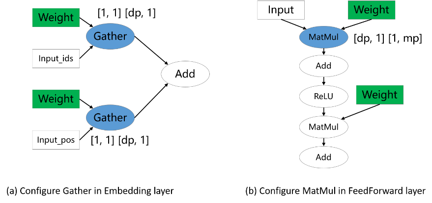
The sharding strategies for parameters are important especially for large models, since parameter-induced memory consumption is the majority of total memory consumption. Therefore, parameter-involved operators usually need to explicitly configure the sharding strategies. In the following examples in the figure, Gather and MatMul involving weights are configured shardings, while other operators are not. These correspond the data-parallel Embedding layer and hybrid-parallel FeedForward Layer in mindformers, respectively.

Configure dimension-manipulation operators

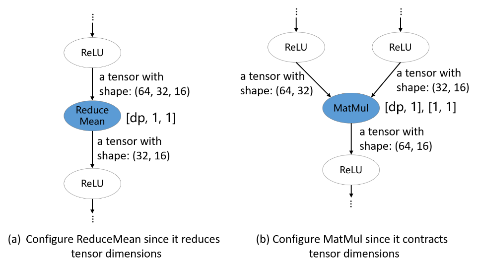
In deep learning frameworks, operators can be broadly classified into two categories: semantically simple dimension-preserving operators and dimension-manipulation operators. Sharding Propagation could easily propagate shardings from inputs to outputs for dimension-preserving operators. However, for dimension-manipulation operators, explicit annotations should be configured to express users’ intuition, to avoid Sharding Propagation to derive non-user-desired shardings. In the following figure, ReduceMean and MatMul operators are configured shardings.

Configure parallelism-changing-boundary operators

For a model like ResNet, different parts of the model may prefer different parallelisms: front part uses data parallelism, while tail part uses model parallelism. This is achieved by annotating parallelism-changing boundary operators. In the example of following figure, the first MatMul propagates the data-parallelism sharding to the front part, while the second MatMul propagates the model-parallelism sharding to the tail part.

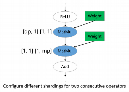
Users should not only understand the main idea of Sharding Propagation, but also have a preferred parallelism for their training models. If there is a sharding strategy inferred by Sharding Propagation that is conflict with your intuition, just add the preferred sharding to the operator. It indeed needs some trial-and-errors to acquire the satisfactory configuration.