Reading IR

Overview

When a model compiled using MindSpore runs in the graph mode context.set_context(mode=context.GRAPH_MODE) and context.set_context(save_graphs=True) is set in the configuration, some intermediate files will be generated during graph compliation. These intermediate files are called IR files. Currently, there are three IR files:

.ir file: An IR file that describes the model structure in text format and can be directly viewed using any text editors.
.dat file: An IR file that describes the model structure more strictly than the .ir file. It contains more contents and can be directly viewed using any text editors.
.dot file: An IR file that describes the topology relationships between different nodes. You can use this file by graphviz as the input to generate images for users to view the model structure. For models with multiple operators, it is recommended using the visualization component MindInsight to visualize computing graphs.

Saving IR

context.set_context(save_graphs=True) is used to save the intermediate code in each compilation phase. The intermediate code can be saved in two formats. One is the text format with the suffix .ir, and the other is the graphical format with the suffix .dot. When the network scale is small, you are advised to use the graphical format that is more intuitive. When the network scale is large, you are advised to use the text format that is more efficient.

You can run the graphviz command to convert a .dot file to the picture format. For example, you can run the dot -Tpng *.dot -o *.png command to convert a .dot file to a .png file.

Add the following code to train.py. When running the script, MindSpore will automatically store the IR files generated during compilation under the specified path.

if __name__ == "__main__":
    context.set_context(save_graphs=True, save_graphs_path="path/to/ir/files")

After the training command is executed, some files are generated in the path of save_graphs_path.

.
├──00_parse_0000.ir
├──00_parse_0001.dat
├──00_parse_0002.dot
├──01_symbol_resolve_0003.ir
├──01_symbol_resolve_0004.dat
├──01_symbol_resolve_0005.dot
├──02_combine_like_graphs_0006.ir
├──02_combine_like_graphs_0007.dat
├──02_combine_like_graphs_0008.dot
├──03_inference_opt_prepare_0009.ir
├──03_inference_opt_prepare_0010.dat
├──03_inference_opt_prepare_0011.dot
├──04_abstract_specialize_0012.ir
├──04_abstract_specialize_0013.dat
├──04_abstract_specialize_0014.dot
...

The IR files starting with digits and underscores are generated during the ME graph compilation. The compute graph is saved in each phase of the pipeline. Let’s see the important phases.

The parse phase parses the construct function of the entrance. If viewing the IR file, we can see that only the graph information of the top cell is parsed in this phase.
The symbol_resolve phase recursively parses other functions and objects directly or indirectly referenced by the entry function. When using the unsupported syntax, it will get an error in this phase.
The abstract_specialize phase infers every node’s data type and shape by the cell’s inputs. When you want to know the shape or data type of a specific operator in IR, you can view this IR file.
The optimize phase, hardware-independent optimization is performed, the automatic differential and automatic parallel functions are also performed. Some ir files with the prefix opt_pass are saved here. No need to pay too much attention to those files if you are not the framework developer.
The validate phase will check the temporary operators which should be removed in the prior phase. If any temporary operator exists, the process will report an error and exit.
The task_emit phase will transfer the compute graph to the backend for further processing.
The execute phase will execute the compute graph. This is the final graph in the phase of frontend.

In addition, you don’t need to pay too much attention to the IR files (such as files beginning with hwopt) if you are not the framework developer because the backend is close to the hardware. Only need pay attention to the file graph_build_[graph_id]_[IR_id].ir. It is the MindIR after the frontend and backend optimization.

Multiple files may be saved because the backend only can handle the single graph. It is different with the frontend when the front save all sub-graphs in the one file.

IR File Contents Introduction

The following is an example to describe the contents of the IR file. The content may have some changes with the version upgrade of MindSpore.

import mindspore.context as context
import mindspore.nn as nn
from mindspore import Tensor
from mindspore import ops
from mindspore import dtype as mstype

context.set_context(mode=context.GRAPH_MODE)
context.set_context(save_graphs=True, save_graphs_path="./")

class Net(nn.Cell):
    def __init__(self):
        super().__init__()
        self.add = ops.Add()
        self.sub = ops.Sub()
        self.mul = ops.Mul()
        self.div = ops.Div()

    def func(x, y):
        return self.div(x, y)

    def construct(self, x, y):
        a = self.sub(x, 1)
        b = self.add(a, y)
        c = self.mul(b, self.func(a, b))
        return c

input1 = Tensor(3, mstype.float32)
input2 = Tensor(2, mstype.float32)
net = Net()
out = net(input1, input2)
print(out)

ir Introduction

Use a text editing software (for example, vi) to open the 04_abstract_specialize_0012.ir file. The file contents are as follows:

#IR entry      : @1_construct_wrapper.21
#attrs         :
#Total params  : 2
  4
%para1_x : <Tensor[Float32]x()>
%para2_y : <Tensor[Float32]x()>
  7
#Total subgraph : 3
  9
subgraph attr:
Undeterminate : 0
subgraph @2_construct.22(%para3_x, %para4_y) {
 %0(a) = Sub(%para3_x, Tensor(shape=[], dtype=Float32, value= 1)) {instance name: sub} primitive_attrs: {input_names: [x, y], output_names: [output]}
     : (<Tensor[Float32]x()>, <Tensor[Float32]x()>) -> (<Tensor[Float32]x()>)
     # In file train.py(34)/        a = self.sub(x, 1)/
 %1(b) = Add(%0, %para4_y) {instance name: add} primitive_attrs: {input_names: [x, y], output_names: [output]}
     : (<Tensor[Float32]x()>, <Tensor[Float32]x()>) -> (<Tensor[Float32]x()>)
     # In file train.py(35)/        b = self.add(a, y)/
 %2([CNode]5) = call @3_func.23(%0, %1)
     : (<Tensor[Float32]x()>, <Tensor[Float32]x()>) -> (<Tensor[Float32]x()>)
     # In file train.py(36)/        c = self.mul(b, self.func(a, b))/
 %3(c) = Mul(%1, %2) {instance name: mul} primitive_attrs: {input_names: [x, y], output_names: [output]}
     : (<Tensor[Float32]x()>, <Tensor[Float32]x()>) -> (<Tensor[Float32]x()>)
     # In file train.py(36)/        c = self.mul(b, self.func(a, b))/
 Return(%3)
     : (<Tensor[Float32]x()>)
     # In file train.py(37)/        return c/
}
 29
subgraph attr:
Undeterminate : 0
subgraph @3_func.23(%para5_x, %para6_y) {
 %0([CNode]20) = Div(%para5_x, %para6_y) {instance name: div} primitive_attrs: {input_names: [x, y], output_names: [output]}
     : (<Tensor[Float32]x()>, <Tensor[Float32]x()>) -> (<Tensor[Float32]x()>)
     # In file train.py(31)/        return self.div(x, y)/
 Return(%0)
     : (<Tensor[Float32]x()>)
     # In file train.py(31)/        return self.div(x, y)/
}
 40
subgraph attr:
subgraph @1_construct_wrapper.21() {
 %0([CNode]2) = call @2_construct.22(%para1_x, %para2_y)
     : (<Tensor[Float32]x()>, <Tensor[Float32]x()>) -> (<Tensor[Float32]x()>)
     # In file train.py(37)/        return c/
 Return(%0)
     : (<Tensor[Float32]x()>)
     # In file train.py(37)/        return c/
}

The above contents can be divided into two parts, the first part is the input list and the second part is the graph structure. The first line tells us the name of the top MindSpore graph about the network, 1_construct_wrapper.21, or the entry graph. Line 3 tells us how many inputs are in the network. Line 5 to 6 are the input list, which is in the format of %para[No.]_[name] : <[data_type]x[shape]>. Line 8 tells us the number of subgraph parsed by the network. There are 3 graphs in this IR. Line 42 is the entry graph 1_construct_wrapper.21. Line 32 is graph 3_func.23, parsed from the func(x, y) in the source script. Line 12 is graph 2_construct.22, parsed from the function construct. Taking graph 2_construct.22 as an example, Line 10 to 28 indicate the graph structure, which contains several nodes, namely, CNode. In this example, there are Sub, Add, Mul. They are defined in the function __init__. Line 19 calls a graph by call @3_func.23. It indicates calling the graph func(x, y) to execute a division operation.

The CNode information format is as follows: including the node name, attribute, input node, the specs of the inputs and outputs, and source code parsing call stack. The ANF graph is a unidirectional acyclic graph. So, the connection between nodes is displayed only based on the input relationship. The corresponding source code reflects the relationship between the CNode and the script source code. For example, line 15 is parsed from a = self.sub(x, 1).

  %[No.]([debug_name]) = [op_name]([arg], ...) primitive_attrs: {[key]: [value], ...}
      : (<[input data_type]x[input shape]>, ...) -> (<[output data_type]x[output shape]>, ...)
      # Corresponding source code

About the corresponding source code:

There are two mode for the corresponding source code displaying. The first mode is to display the complete call stack, such as 15_execute_0141.ir on the frontend and graph_build_0_136.ir on the backend. The second mode only displays one code line for reducing the size of the IR file, which eliminates the call stack, such as 04_abstract_specialize_0012.ir.
If the operator is a back propagation operator, the associated code line will not only display its own code, but also the corresponding forward code, identified by “Corresponding forward node candidate:”.
If the operator is a fusion operator, the associated code line will display the fusion related code, identified by “Corresponding code candidate:”, where the separator “-” is used to distinguish different codes.

After several optimizations by the compiler, the node may undergo several changes (such as operator splitting and operator merging). The source code parsing call stack information of the node may not be in a one-to-one correspondence with the script. This is only an auxiliary method.

After the kernel select phase at the backend, two lines of input and output specification information (that is, the content after :) will appear. The first line represents the specifications on the HOST side, and the second line represents the specifications on the DEVICE side.

dat Introduction

Use a text editing software (for example, vi) to open the 04_abstract_specialize_0013.dat file. The file contents are as follows:

# [No.1] 1_construct_wrapper.21
# In file train.py(33)/    def construct(self, x, y):/
funcgraph fg_21(
       %para1 : Tensor(F32)[]    # x
       , %para2 : Tensor(F32)[]    # y
   ) {
   %1 : Tensor(F32)[] = FuncGraph::fg_22(%para1, %para2)    #(Tensor(F32)[], Tensor(F32)[])    # fg_22=2_construct.22 #scope: Default
     # In file train.py(37)/        return c/#[CNode]2
   Primitive::Return{prim_type=1}(%1)    #(Tensor(F32)[]) #scope: Default
     # In file train.py(37)/        return c/#[CNode]1
}
# order:
#   1: 1_construct_wrapper.21:[CNode]2{[0]: ValueNode<FuncGraph> 2_construct.22, [1]: x, [2]: y}
#   2: 1_construct_wrapper.21:[CNode]1{[0]: ValueNode<Primitive> Return, [1]: [CNode]2}
 15
 16
# [No.2] 2_construct.22
# In file train.py(33)/    def construct(self, x, y):/
funcgraph fg_22(
       %para3 : Tensor(F32)[]    # x
       , %para4 : Tensor(F32)[]    # y
   ) {
   %1 : Tensor(F32)[] = PrimitivePy::Sub{prim_type=2}[input_names=["x", "y"], output_names=["output"]](%para3, Tensor(43)[])    #(Tensor(F32)[], Tenso    r(F32)[]) #scope: Default
     # In file train.py(34)/        a = self.sub(x, 1)/#a
   %2 : Tensor(F32)[] = PrimitivePy::Add{prim_type=2}[input_names=["x", "y"], output_names=["output"]](%1, %para4)    #(Tensor(F32)[], Tensor(F32)[])     #scope: Default
     # In file train.py(35)/        b = self.add(a, y)/#b
   %3 : Tensor(F32)[] = FuncGraph::fg_23(%1, %2)    #(Tensor(F32)[], Tensor(F32)[])    # fg_23=3_func.23 #scope: Default
     # In file train.py(36)/        c = self.mul(b, self.func(a, b))/#[CNode]5
   %4 : Tensor(F32)[] = PrimitivePy::Mul{prim_type=2}[input_names=["x", "y"], output_names=["output"]](%2, %3)    #(Tensor(F32)[], Tensor(F32)[]) #sco    pe: Default
     # In file train.py(36)/        c = self.mul(b, self.func(a, b))/#c
   Primitive::Return{prim_type=1}(%4)    #(Tensor(F32)[]) #scope: Default
     # In file train.py(37)/        return c/#[CNode]4
}
# order:
#   1: 2_construct.22:a{[0]: ValueNode<PrimitivePy> Sub, [1]: x, [2]: ValueNode<Tensor> Tensor(shape=[], dtype=Float32, value= 1)}
#   2: 2_construct.22:b{[0]: ValueNode<PrimitivePy> Add, [1]: a, [2]: y}
#   3: 2_construct.22:[CNode]5{[0]: ValueNode<FuncGraph> 3_func.23, [1]: a, [2]: b}
#   4: 2_construct.22:c{[0]: ValueNode<PrimitivePy> Mul, [1]: b, [2]: [CNode]5}
#   5: 2_construct.22:[CNode]4{[0]: ValueNode<Primitive> Return, [1]: c}
 40
 41
# [No.3] 3_func.23
# In file train.py(30)/    def func(x, y):/
funcgraph fg_23(
       %para5 : Tensor(F32)[]    # x
       , %para6 : Tensor(F32)[]    # y
   ) {
   %1 : Tensor(F32)[] = PrimitivePy::Div{prim_type=2}[input_names=["x", "y"], output_names=["output"]](%para5, %para6)    #(Tensor(F32)[], Tensor(F32)    []) #scope: Default
     # In file train.py(31)/        return self.div(x, y)/#[CNode]20
   Primitive::Return{prim_type=1}(%1)    #(Tensor(F32)[]) #scope: Default
     # In file train.py(31)/        return self.div(x, y)/#[CNode]19
}
# order:
#   1: 3_func.23:[CNode]20{[0]: ValueNode<PrimitivePy> Div, [1]: x, [2]: y}
#   2: 3_func.23:[CNode]19{[0]: ValueNode<Primitive> Return, [1]: [CNode]20}
 56
 57
# num of total function graphs: 3

Above, it lists all the graphs beginning with the entry graph. Line 1 indicates graph 1_construct_wrapper.21 whose id is No.1. And line 7 calls graph 2_construct.22. line 17 to 39 shows the information of graph 2_construct.22. Taking graph 2_construct.22 as an example. Line 18 tells us which function this graph is parsed from. Line 20 to 21 indicates the input information which is in the format of %para[No.] : [data_type][shape] # [name]. Line 23 to 32 indicates the graph structure, which contains several nodes, namely, CNode. In this example, there are Sub, Add, Mul. They are defined in the function __init__. Line 34 to 39 shows the execution order of the CNode from graph 2_construct.22, corresponding to the order of code execution. The information format is: No.: belonging graph:node name{[0]: the first input, [1]: the second input, ...}. For CNode, the first input indicates how to compute for this CNode. Line 28 indicates the number of graphs. Here is 3.

The CNode information format is as follows: including the node name, attribute, input node, output information, format and the corresponding source code.

%[No,] : [outputs' Spec] = [op_name]{[prim_type]}[attr0, attr1, ...](arg0, arg1, ...)    #(inputs' Spec)#[scope]
  # Corresponding source code/#debug_name

dot Introduction

We can use this file by graphviz as the input to generate images for users to view the model structure. For example, under the Linux operating system, we can convert a PNG image by the following command.

dot -Tpng -o 04_abstract_specialize_0014.png 04_abstract_specialize_0014.dot

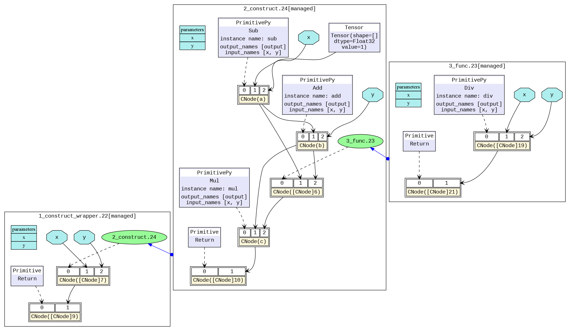
The transformed image is shown below, and we can visually see the model structure. The Different black boxes distinguish different subgraphs, and the blue arrows between graphs represent calling another graph. The blue area represents the parameter, the rectangle represents the parameter list of the graph, the hexagon and the black arrow represent the parameter as the input of the CNode to participate in the calculation process. The yellow rectangle represents the CNode. As can be seen from the picture, the CNode input starts from index 0, and the 0th input (that is, the purple or green area) represents what calculation the operator will perform, which is connected by a dotted arrow. The type is usually an operator primitive, or it can also be another graph. The rest inputs are the parameters required for the calculation.

For models with multiple operators, the picture will be very large. It is recommended using the visualization component MindInsight to visualize computing graphs.

Reading analyze_fail.dat

In the process of MindSpore compiling a graph, the exceptions about graph evaluating fail usually happen. But we can find the reason by analyzing the exception information and analyze_fail.dat.

For example, we run the script below.

import mindspore.context as context
import mindspore.nn as nn
from mindspore import Tensor
from mindspore.nn import Cell
from mindspore import ops
from mindspore import dtype as mstype
  7
context.set_context(mode=context.GRAPH_MODE)
context.set_context(save_graphs=True)
 10
class Net(nn.Cell):
   def __init__(self):
       super().__init__()
       self.add = ops.Add()
       self.sub = ops.Sub()
       self.mul = ops.Mul()
       self.div = ops.Div()
 18
   def func(x, y):
       return self.div(x, y)
 21
   def construct(self, x, y):
       a = self.sub(x, 1)
       b = self.add(a, y)
       c = self.mul(b, self.func(a, a, b))
       return c
 27
input1 = Tensor(3, mstype.float32)
input2 = Tensor(2, mstype.float32)
net = Net()
out = net(input1, input2)
print(out)

An error happens.

[EXCEPTION] ANALYZER(31946,7f6f03941740,python):2021-09-18-15:10:49.094.863 [mindspore/ccsrc/pipeline/jit/static_analysis/stack_frame.cc:85] DoJump] The parameters number of the function is 2, but the number of provided arguments is 3.
FunctionGraph ID : func.18
NodeInfo: In file test.py(19)
   def func(x, y):
  5
Traceback (most recent call last):
 File "test.py", line 31, in <module>
   out = net(input1, input2)
 File "/home/workspace/mindspore/mindspore/nn/cell.py", line 404, in __call__
   out = self.compile_and_run(*inputs)
 File "/home/workspace/mindspore/mindspore/nn/cell.py", line 682, in compile_and_run
   self.compile(*inputs)
 File "/home/workspace/mindspore/mindspore/nn/cell.py", line 669, in compile
   _cell_graph_executor.compile(self, *inputs, phase=self.phase, auto_parallel_mode=self._auto_parallel_mode)
 File "/home/workspace/mindspore/mindspore/common/api.py", line 542, in compile
   result = self._graph_executor.compile(obj, args_list, phase, use_vm, self.queue_name)
TypeError: mindspore/ccsrc/pipeline/jit/static_analysis/stack_frame.cc:85 DoJump] The parameters number of the function is 2, but the number of provided arguments is 3.
FunctionGraph ID : func.18
NodeInfo: In file test.py(19)
   def func(x, y):
 21
The function call stack (See file '/home/workspace/mindspore/rank_0/om/analyze_fail.dat' for more details):
# 0 In file test.py(26)
       return c
       ^
# 1 In file test.py(25)
       c = self.mul(b, self.func(a, a, b))
                       ^

Above exception is ‘TypeError: mindspore/ccsrc/pipeline/jit/static_analysis/stack_frame.cc:85 DoJump] The parameters number of the function is 2, but the number of provided arguments is 3…’. And it tells us FunctionGraph ID : func.18 only needs two parameters, but actually gives 3. We can find the related code is self.func(a, a, b) from ‘The function call stack … In file test.py(25)’. Easily, by checking the code, we know that we gave too much parameter to the calling function.

Sometimes the exception information is not enough easy to understand. Or we want to see the part of graph information that have evaluated. Then we can open /home/workspace/mindspore/rank_0/om/analyze_fail.dat that indicated in the exception text by using a text editing software (for example, vi).

# [No.1] construct_wrapper.0
# In file test.py(22)/    def construct(self, x, y):/
funcgraph fg_0(
       %para1 : Tensor(F32)[]    # x
       , %para2 : Tensor(F32)[]    # y
   ) {
  7
#------------------------> 0
   %1 = FuncGraph::fg_3(%para1, %para2)    #(Tensor(F32)[], Tensor(F32)[])    # fg_3=construct.3 #scope: Default
     # In file test.py(26)/        return c/#[CNode]2
   Primitive::Return{prim_type=1}(%1)    #(Undefined) #scope: Default
     # In file test.py(26)/        return c/#[CNode]1
}
# order:
#   1: construct_wrapper.0:[CNode]2{[0]: ValueNode<FuncGraph> construct.3, [1]: x, [2]: y}
#   2: construct_wrapper.0:[CNode]1{[0]: ValueNode<Primitive> Return, [1]: [CNode]2}
 17
 18
# [No.2] construct.3
# In file test.py(22)/    def construct(self, x, y):/
funcgraph fg_3(
       %para3 : Tensor(F32)[]    # x
       , %para4 : Tensor(F32)[]    # y
   ) {
   %1 : Tensor(F32)[] = DoSignaturePrimitive::S-Prim-Sub{prim_type=1}[input_names=["x", "y"], output_names=["output"]](%para3, I64(1))    #(Tensor(F32)[], I64) #scope: Default
     # In file test.py(23)/        a = self.sub(x, 1)/#a
   %2 : Tensor(F32)[] = DoSignaturePrimitive::S-Prim-Add{prim_type=1}[input_names=["x", "y"], output_names=["output"]](%1, %para4)    #(Tensor(F32)[], Tensor(F32)[]) #scope: Default
     # In file test.py(24)/        b = self.add(a, y)/#b
 29
#------------------------> 1
   %3 = FuncGraph::fg_18(%1, %1, %2)    #(Tensor(F32)[], Tensor(F32)[], Tensor(F32)[])    # fg_18=func.18 #scope: Default
     # In file test.py(25)/        c = self.mul(b, self.func(a, a, b))/#[CNode]5
   %4 = DoSignaturePrimitive::S-Prim-Mul{prim_type=1}[input_names=["x", "y"], output_names=["output"]](%2, %3)    #(Tensor(F32)[], Undefined) #scope: Default
     # In file test.py(25)/        c = self.mul(b, self.func(a, a, b))/#c
   Primitive::Return{prim_type=1}(%4)    #(Undefined) #scope: Default
     # In file test.py(26)/        return c/#[CNode]4
}
# order:
#   1: construct.3:a{[0]: a, [1]: ValueNode<Int64Imm> 1, [2]: ValueNode<Float> Float32}
#   2: construct.3:a{[0]: ValueNode<DoSignaturePrimitive> S-Prim-Sub, [1]: x, [2]: ValueNode<Int64Imm> 1}
#   3: construct.3:b{[0]: ValueNode<DoSignaturePrimitive> S-Prim-Add, [1]: a, [2]: y}
#   4: construct.3:[CNode]5{[0]: ValueNode<FuncGraph> func.18, [1]: a, [2]: a, [3]: b}
#   5: construct.3:c{[0]: ValueNode<DoSignaturePrimitive> S-Prim-Mul, [1]: b, [2]: [CNode]5}
#   6: construct.3:[CNode]4{[0]: ValueNode<Primitive> Return, [1]: c}
 45
 46
#===============================================================================
# num of function graphs in stack: 2

The file analyze_fail.dat has the same information format with the file .dat. The only difference is analyze_fail.dat will locate the node which inferring failed. Searching the point by the text of ------------------------>, we reach the last position of the ------------------------> 1 at line 30. The node at line 31 to 32 have an error. Its IR expression is %3 = FuncGraph::fg_18(%1, %1, %2) .... We can know the node have 3 parameters from (%1, %1, %2). But actually the function only need 2. So the compiler will fail when evaluating the node. To solve th problem, we should decrease the parameter number.