Training Process Visualization

Overview

Scalars, images, computational graphs, and model hyperparameters during training are recorded in files and can be viewed on the web page.

Operation Process

Prepare a training script, specify scalars, images, computational graphs, and model hyperparameters in the training script, record them in the summary log file, and run the training script.
Start MindInsight and specify the summary log file directory using startup parameters. After MindInsight is started, access the visualization page based on the IP address and port number. The default access IP address is http://127.0.0.1:8080.
During the training, when data is written into the summary log file, you can view the data on the web page.

Preparing the Training Script

Collect Summary Data

Currently, MindSpore uses the Callback mechanism to save scalars, images, computational graphs, and model hyperparameters to summary log files and display them on the web page.

Scalar and image data is recorded by using the Summary operator. A computational graph is saved to the summary log file by using SummaryRecord after network compilation is complete. Model parameters are saved to the summary log file by using TrainLineage or EvalLineage.

Step 1: Call the Summary operator in the construct function of the derived class that inherits nn.Cell to collect image or scalar data.

For example, when a network is defined, image data is recorded in construct of the network. When the loss function is defined, the loss value is recorded in construct of the loss function.

Record the dynamic learning rate in construct of the optimizer when defining the optimizer.

The sample code is as follows:

from mindspore import context, Tensor, nn
from mindspore.common import dtype as mstype
from mindspore.ops import operations as P
from mindspore.ops import functional as F
from mindspore.nn import Optimizer


class CrossEntropyLoss(nn.Cell):
    """Loss function definition."""
    def __init__(self):
        super(CrossEntropyLoss, self).__init__()
        self.cross_entropy = P.SoftmaxCrossEntropyWithLogits()
        self.mean = P.ReduceMean()
        self.one_hot = P.OneHot()
        self.on_value = Tensor(1.0, mstype.float32)
        self.off_value = Tensor(0.0, mstype.float32)

        # Init ScalarSummary
        self.sm_scalar = P.ScalarSummary()

    def construct(self, logits, label):
        label = self.one_hot(label, F.shape(logits)[1], self.on_value, self.off_value)
        loss = self.cross_entropy(logits, label)[0]
        loss = self.mean(loss, (-1,))

        # Record loss
        self.sm_scalar("loss", loss)
        return loss


class MyOptimizer(Optimizer):
    """Optimizer definition."""
    def __init__(self, learning_rate, params, ......):
        ......
        # Initialize ScalarSummary
        self.sm_scalar = P.ScalarSummary()
        self.histogram_summary = P.HistogramSummary()
        self.weight_names = [param.name for param in self.parameters]

    def construct(self, grads):
        ......
        # Record learning rate here
        self.sm_scalar("learning_rate", learning_rate)

        # Record weight
        self.histogram_summary(self.weight_names[0], self.paramters[0])
        # Record gradient
        self.histogram_summary(self.weight_names[0] + ".gradient", grads[0])

        ......


class Net(nn.Cell):
    """Net definition."""
    def __init__(self):
        super(Net, self).__init__()
        ......

        # Init ImageSummary
        self.sm_image = P.ImageSummary()

    def construct(self, data):
        # Record image by Summary operator
        self.sm_image("image", data)
        ......
        return out

Step 2: Use the Callback mechanism to add the required callback instance to specify the data to be recorded during training.

SummaryStep specifies the step interval for recording summary data.
TrainLineage records parameters related to model training.
EvalLineage records parameters related to the model test.

The network parameter needs to be specified when SummaryRecord is called to record the computational graph. By default, the computational graph is not recorded.

The sample code is as follows:

from mindinsight.lineagemgr import TrainLineage, EvalLineage
from mindspore import Model, nn, context
from mindspore.train.callback import SummaryStep
from mindspore.train.summary.summary_record import SummaryRecord


def test_summary():
    # Init context env
    context.set_context(mode=context.GRAPH_MODE, device_target='Ascend')
    # Init hyperparameter
    epoch = 2
    # Init network and Model
    net = Net()
    loss_fn = CrossEntropyLoss()
    optim = MyOptimizer(learning_rate=0.01, params=network.trainable_params())
    model = Model(net, loss_fn=loss_fn, optimizer=optim, metrics=None)

    # Init SummaryRecord and specify a folder for storing summary log files
    # and specify the graph that needs to be recorded
    with SummaryRecord(log_dir='./summary', network=net) as summary_writer:
        summary_callback = SummaryStep(summary_writer, flush_step=10)

        # Init TrainLineage to record the training information
        train_callback = TrainLineage(summary_writer)

        # Prepare mindrecord_dataset for training
        train_ds = create_mindrecord_dataset_for_training()
        model.train(epoch, train_ds, callbacks=[summary_callback, train_callback])

        # Init EvalLineage to record the evaluation information
        eval_callback = EvalLineage(summary_writer)

        # Prepare mindrecord_dataset for testing
        eval_ds = create_mindrecord_dataset_for_testing()
        model.eval(eval_ds, callbacks=[eval_callback])

Use the save_graphs option of context to record the computational graph after operator fusion. ms_output_after_hwopt.pb is the computational graph after operator fusion.

Currently MindSpore supports recording computational graph after operator fusion for Ascend 910 AI processor only.

It’s recommended that you reduce calls to HistogramSummary under 10 times per batch. The more you call HistogramSummary, the more performance overhead.

Please use the with statement to ensure that SummaryRecord is properly closed at the end, otherwise the process may fail to exit.

Collect Performance Profile Data

To enable the performance profiling of neural networks, MindInsight Profiler APIs should be added into the script. At first, the MindInsight Profiler object need to be set after set context and before the network initialization. Then, at the end of the training, Profiler.analyse() should be called to finish profiling and generate the perforamnce analyse results.

The sample code is as follows:

from mindinsight.profiler import Profiler
from mindspore import Model, nn, context


def test_profiler():
    # Init context env
    context.set_context(mode=context.GRAPH_MODE, device_target='Ascend', device_id=int(os.environ["DEVICE_ID"]))

    # Init Profiler
    profiler = Profiler(output_path='./data', is_detail=True, is_show_op_path=False, subgraph='all')

    # Init hyperparameter
    epoch = 2
    # Init network and Model
    net = Net()
    loss_fn = CrossEntropyLoss()
    optim = MyOptimizer(learning_rate=0.01, params=network.trainable_params())
    model = Model(net, loss_fn=loss_fn, optimizer=optim, metrics=None)
    # Prepare mindrecord_dataset for training
    train_ds = create_mindrecord_dataset_for_training()
    # Model Train
    model.train(epoch, train_ds)

    # Profiler end
    profiler.analyse()

MindInsight Commands

View the command help information.

mindinsight --help

View the version information.

mindinsight --version

Start the service.

mindinsight start [-h] [--config <CONFIG>] [--workspace <WORKSPACE>]
                  [--port <PORT>] [--reload-interval <RELOAD_INTERVAL>]
                  [--summary-base-dir <SUMMARY_BASE_DIR>]

Optional parameters as follows:

-h, --help : Displays the help information about the startup command.
--config <CONFIG> : Specifies the configuration file or module. CONFIG indicates the physical file path (file:/path/to/config.py), or a module path (python:path.to.config.module) that can be identified by Python.
--workspace <WORKSPACE> : Specifies the working directory. The default value of WORKSPACE is $HOME/mindinsight.
--port <PORT> : Specifies the port number of the web visualization service. The value ranges from 1 to 65535. The default value of PORT is 8080.
--reload-interval <RELOAD_INTERVAL> : Specifies the interval (unit: second) for loading data. The value 0 indicates that data is loaded only once. The default value of RELOAD_INTERVAL is 3 seconds.
--summary-base-dir <SUMMARY_BASE_DIR> : Specifies the root directory for loading training log data. MindInsight traverses the direct subdirectories in this directory and searches for log files. If a direct subdirectory contains log files, it is identified as the log file directory. If a root directory contains log files, it is identified as the log file directory. SUMMARY_BASE_DIR is the current directory path by default.

When the service is started, the parameter values of the command line are saved as the environment variables of the process and start with MINDINSIGHT_, for example, MINDINSIGHT_CONFIG, MINDINSIGHT_WORKSPACE, and MINDINSIGHT_PORT.

Stop the service.

mindinsight stop [-h] [--port PORT]

Optional parameters as follows:

-h, --help : Displays the help information about the stop command.
--port <PORT> : Specifies the port number of the web visualization service. The value ranges from 1 to 65535. The default value of PORT is 8080.

View the service process information.

MindInsight provides user with web services. Run the following command to view the running web service process:

ps -ef | grep mindinsight

Run the following command to access the working directory WORKSPACE corresponding to the service process based on the service process ID:

lsof -p <PID> | grep access

Output with the working directory WORKSPACE as follows:

gunicorn  <PID>  <USER>  <FD>  <TYPE>  <DEVICE>  <SIZE/OFF>  <NODE>  <WORKSPACE>/log/gunicorn/access.log

Visualization Components

Training Dashboard

Access the Training Dashboard by selecting a specific training from the training list.

Scalar Visualization

Scalar visualization is used to display the change trend of scalars during training.

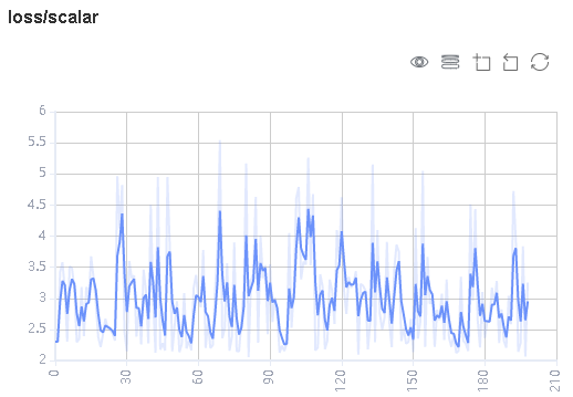
Figure 1: Scalar trend chart

Figure 1 shows a change process of loss values during the neural network training. The horizontal coordinate indicates the training step, and the vertical coordinate indicates the loss value.

Buttons from left to right in the upper right corner of the figure are used to display the chart in full screen, switch the Y-axis scale, enable or disable the rectangle selection, roll back the chart step by step, and restore the chart.

Full-screen Display: Display the scalar curve in full screen. Click the button again to restore it.
Switch Y-axis Scale: Perform logarithmic conversion on the Y-axis coordinate.
Enable/Disable Rectangle Selection: Draw a rectangle to select and zoom in a part of the chart. You can perform rectangle selection again on the zoomed-in chart.
Step-by-step Rollback: Cancel operations step by step after continuously drawing rectangles to select and zooming in the same area.
Restore Chart: Restore a chart to the original state.

Figure 2: Scalar visualization function area

Figure 2 shows the scalar visualization function area, which allows you to view scalar information by selecting different tags, different dimensions of the horizontal axis, and smoothness.

Tag: Select the required tags to view the corresponding scalar information.
Horizontal Axis: Select any of Step, Relative Time, and Absolute Time as the horizontal axis of the scalar curve.
Smoothness: Adjust the smoothness to smooth the scalar curve.
Scalar Synthesis: Synthesize two scalar curves and display them in a chart to facilitate comparison between the two curves or view the synthesized chart.

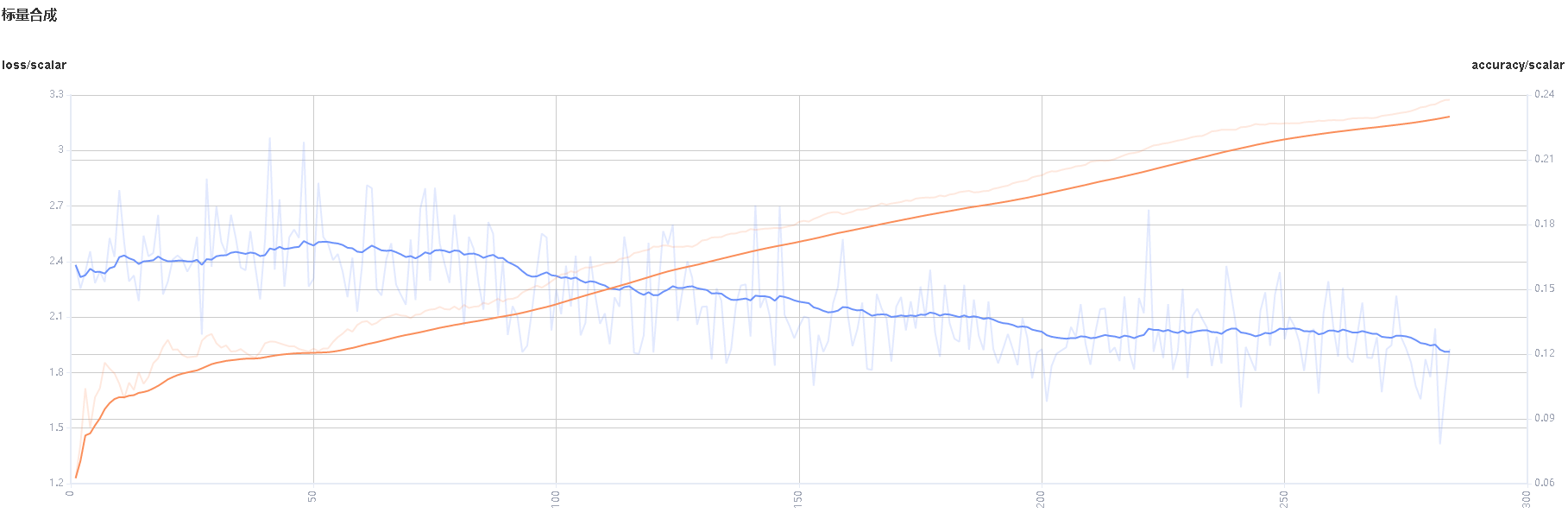
Figure 3: Scalar synthesis of Accuracy and Loss curves

Figure 3 shows the scalar synthesis of the Accuracy and Loss curves. The function area of scalar synthesis is similar to that of scalar visualization. Different from the scalar visualization function area, the scalar synthesis function allows you to select a maximum of two tags at a time to synthesize and display their curves.

Parameter Distribution Visualization

The parameter distribution in a form of a histogram displays tensors specified by a user.

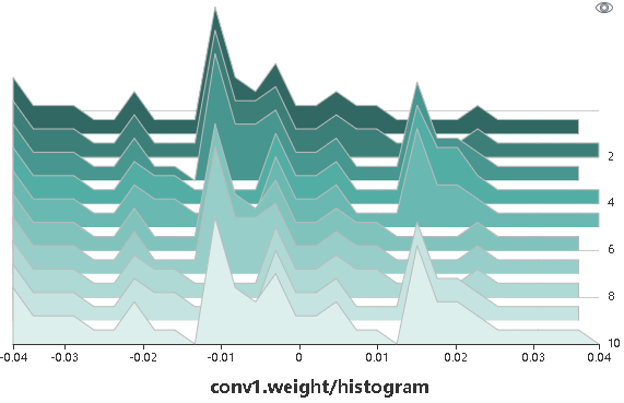
Figure 4: Histogram

Figure 4 shows tensors recorded by a user in a form of a histogram. Click the upper right corner to zoom in the histogram.

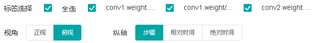
Figure 5: Function area of the parameter distribution histogram

Figure 5 shows the function area of the parameter distribution histogram, including:

Tag selection: Select the required tags to view the corresponding histogram.
Vertical axis: Select any of Step, Relative time, and Absolute time as the data displayed on the vertical axis of the histogram.
Angle of view: Select either Front or Top. Front view refers to viewing the histogram from the front view. In this case, data between different steps is overlapped. Top view refers to viewing the histogram at an angle of 45 degrees. In this case, data between different steps can be presented.

Computational Graph Visualization

Computational graph visualization is used to display the graph structure, data flow direction, and control flow direction of a computational graph. It supports visualization of summary log files and pb files generated by save_graphs configuration in context.

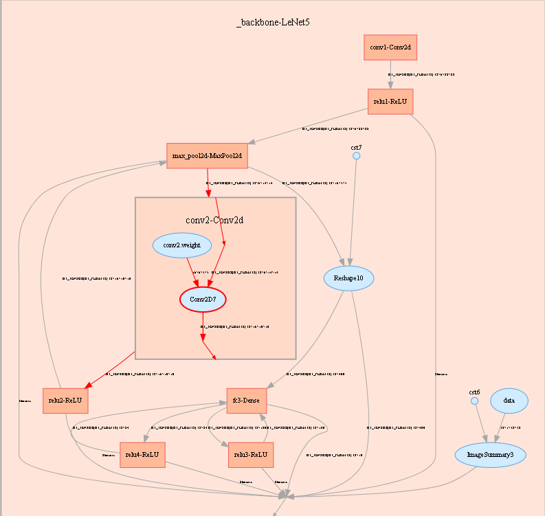
Figure 6: Computational graph display area

Figure 6 shows the network structure of a computational graph. As shown in the figure, select an operator in the area of the display area. The operator has two inputs and one outputs (the solid line indicates the data flow direction of the operator).

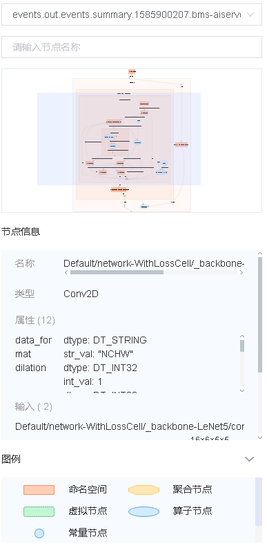
Figure 7: Computational graph function area

Figure 7 shows the function area of the computational graph, including:

File selection box: View the computational graphs of different files.
Search box: Enter a node name and press Enter to view the node.
Thumbnail: Display the thumbnail of the entire network structure. When viewing an extra large image structure, you can view the currently browsed area.
Node information: Display the basic information of the selected node, including the node name, properties, input node, and output node.
Legend: Display the meaning of each icon in the computational graph.

Dataset Graph Visualization

Dataset graph visualization is used to display data processing and augmentation information of a single model training.

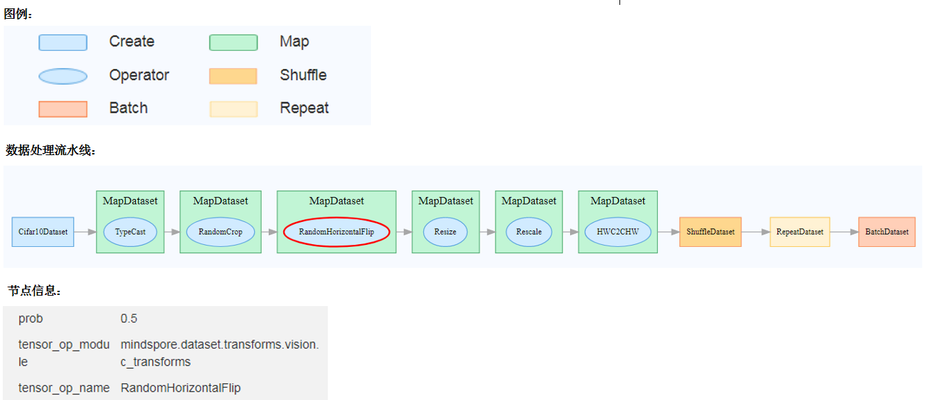
Figure 8: Dataset graph function area

Figure 8 shows the dataset graph function area which includes the following content:

Legend: Display the meaning of each icon in the data lineage graph.
Data Processing Pipeline: Display the data processing pipeline used for training. Select a single node in the graph to view details.
Node Information: Display basic information about the selected node, including names and parameters of the data processing and augmentation operators.

Image Visualization

Image visualization is used to display images specified by users.

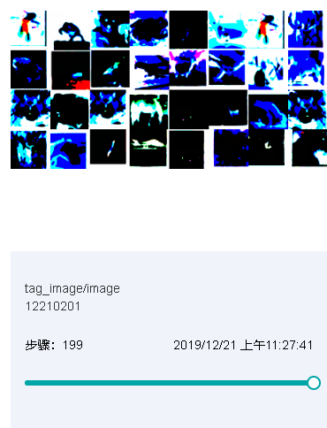
Figure 9: Image visualization

Figure 9 shows how to view images of different steps by sliding the Step slider.

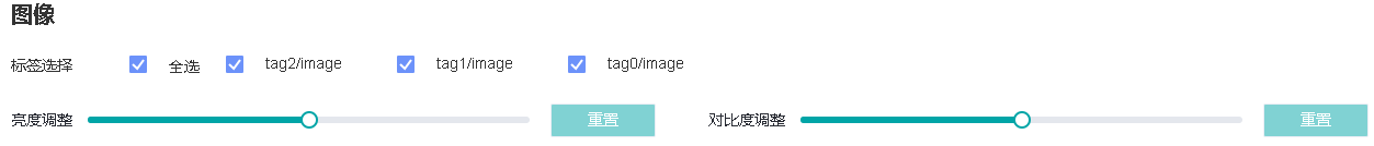
Figure 10: Image visualization function area

Figure 10 shows the function area of image visualization. You can view image information by selecting different tags, brightness, and contrast.

Tag: Select the required tags to view the corresponding image information.
Brightness Adjustment: Adjust the brightness of all displayed images.
Contrast Adjustment: Adjust the contrast of all displayed images.

Model Lineage

Model lineage visualization is used to display the parameter information of all training models.

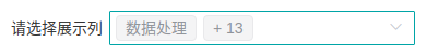
Figure 11: Model parameter selection area

Figure 11 shows the model parameter selection area, which lists the model parameter tags that can be viewed. You can select required tags to view the corresponding model parameters.

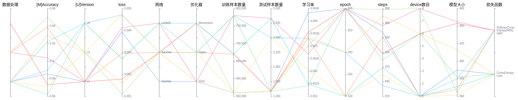
Figure 12: Model lineage function area

Figure 12 shows the model lineage function area, which visualizes the model parameter information. You can select a specific area in the column to display the model information within the area.

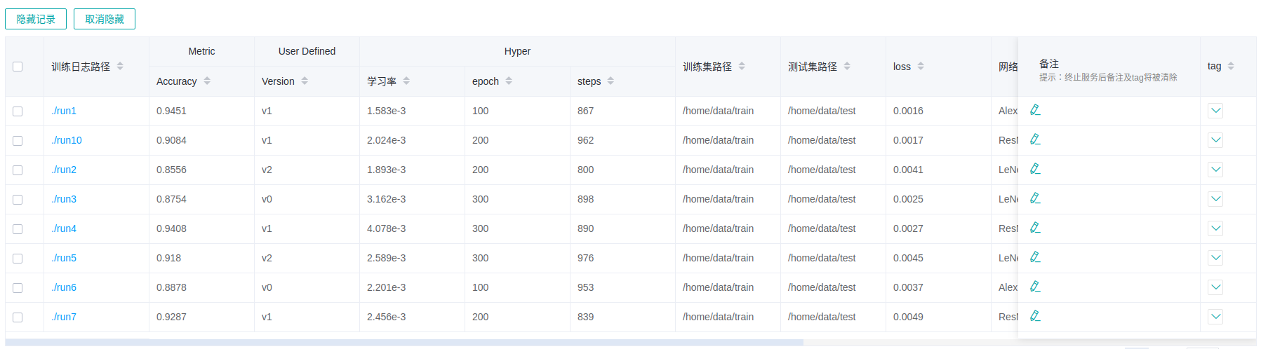
Figure 13: Model list

Figure 13 shows all model information in groups. You can sort the model information in ascending or descending order by specified column.

Dataset Lineage

Dataset lineage visualization is used to display data processing and augmentation information of all model trainings.

Figure 14: Data processing and augmentation operator selection area

Figure 14 shows the data processing and augmentation operator selection area, which lists names of data processing and augmentation operators that can be viewed. You can select required tags to view related parameters.

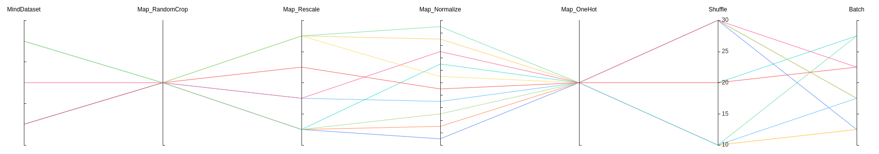
Figure 15: Dataset lineage function area

Figure 15 shows the dataset lineage function area, which visualizes the parameter information used for data processing and augmentation. You can select a specific area in the column to display the parameter information within the area.

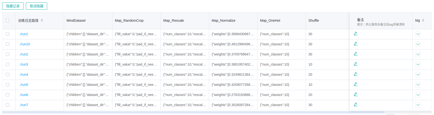
Figure 16: Dataset lineage list

Figure 16 shows the data processing and augmentation information of all model trainings.

Scalars Comparision

Scalars Comparision can be used to compare scalar curves between multiple trainings

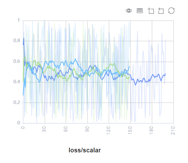
Figure 17: Scalars comparision curve area

Figure 17 shows the scalar curve comparision between multiple trainings. The horizontal coordinate indicates the training step, and the vertical coordinate indicates the scalar value.

Buttons from left to right in the upper right corner of the figure are used to display the chart in full screen, switch the Y-axis scale, enable or disable the rectangle selection, roll back the chart step by step, and restore the chart.

Full-screen Display: Display the scalar curve in full screen. Click the button again to restore it.
Switch Y-axis Scale: Perform logarithmic conversion on the Y-axis coordinate.
Enable/Disable Rectangle Selection: Draw a rectangle to select and zoom in a part of the chart. You can perform rectangle selection again on the zoomed-in chart.
Step-by-step Rollback: Cancel operations step by step after continuously drawing rectangles to select and zooming in the same area.
Restore Chart: Restore a chart to the original state.

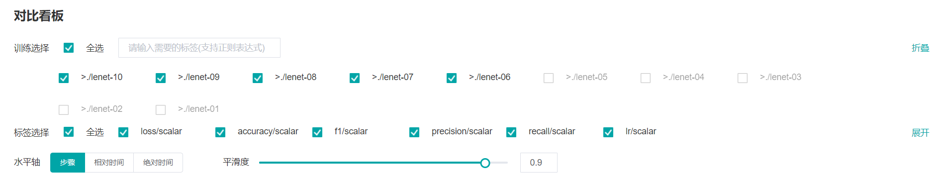
Figure 18: Scalars comparision function area

Figure 18 shows the scalars comparision function area, which allows you to view scalar information by selecting different trainings or tags, different dimensions of the horizontal axis, and smoothness.

Training: Select or filter the required trainings to view the corresponding scalar information.
Tag: Select the required tags to view the corresponding scalar information.
Horizontal Axis: Select any of Step, Relative Time, and Absolute Time as the horizontal axis of the scalar curve.
Smoothness: Adjust the smoothness to smooth the scalar curve.

Performance Profiler

Access the Performance Profiler by selecting a specific training from the training list.

Operator Performance Analysis

The operator performance analysis component is used to display the execution time of the operators during MindSpore run.

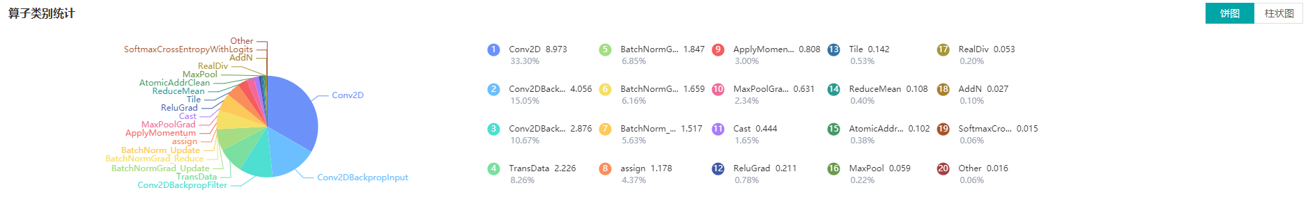
Figure 19: Statistics for Operator Types

Figure 19 displays the statistics for the operator types, including:

Choose pie or bar graph to show the proportion time occupied by each operator type. The time of one operator type is calculated by accumulating the execution time of operators belong to this type.
Display top 20 operator types with longest execution time, show the proportion and execution time (ms) of each operator type.

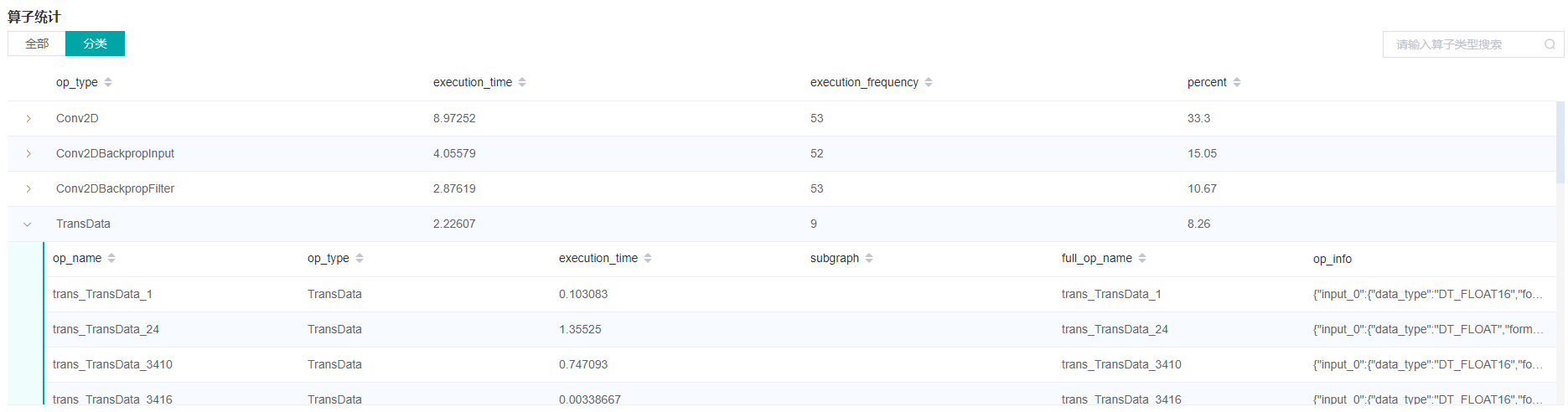
Figure 20: Statistics for Operators

Figure 20 displays the statistics table for the operators, including:

Choose All: Display statistics for the operators, including operator name、type、excution time、full scope time、information etc. The table will be sorted by execution time by default.
Choose Type: Display statistics for the operator types, including operator type name、execution time、execution frequency and proportion of total time. Users can click on each line, querying for all the operators belong to this type.
Search: There is a search box on the right, which can support fuzzy search for operators/operator types.

Specifications

To limit time of listing summaries, MindInsight lists at most 999 summary items.

To limit memory usage, MindInsight limits the number of tags and steps:

There are 300 tags at most in each training dashboard. Total number of scalar tags, image tags, computation graph tags, parameter distribution(histogram) tags can not exceed 300. Specially, there are 10 computation graph tags at most. When tags exceed limit, MindInsight preserves the most recently processed tags.
There are 1000 steps at most for each scalar tag in each training dashboard. When steps exceed limit, MindInsight will sample steps randomly to meet this limit.
There are 10 steps at most for each image tag in each training dashboard. When steps exceed limit, MindInsight will sample steps randomly to meet this limit.
There are 50 steps at most for each parameter distribution(histogram) tag in each training dashboard. When steps exceed limit, MindInsight will sample steps randomly to meet this limit.

To ensure performance, MindInsight implements scalars comparision with the cache mechanism and the following restrictions:

The scalars comparision supports only for trainings in cache.
The maximum of 15 latest trainings (sorted by modification time) can be retained in the cache.
The maximum of 5 trainings can be selected for scalars comparision at the same time.

To limit the data size generated by the Profiler, MindInsight suggests that for large neural network, the profiled steps should better below 10.