Model Security

Overview

This tutorial describes the model security protection methods provided by MindArmour, helping you quickly use MindArmour and provide certain security protection capabilities for your AI model.

At the beginning of AI algorithm design, related security threats are sometimes not considered. As a result, the developed AI model may easily be affected by malicious attackers, leading to inaccurate judgment of the AI system. An attacker adds small perturbations that are not easily perceived by human to the original sample, causing deep learning model misjudgment. This is called an adversarial example attack. MindArmour model security toolkit provides functions such as adversarial example generation, adversarial example detection, model defense, and attack/defense effect evaluation, providing important support for AI model security research and AI application security.

The adversarial example generation module enables security engineers to quickly and efficiently generate adversarial examples for attacking AI models.
The adversarial example detection and defense modules allow users to detect and filter adversarial examples and enhance the robustness of AI models to adversarial examples.
The evaluation module provides multiple metrics to comprehensively evaluate the attack and defense performance of adversarial examples.

This section describes how to use MindArmour in adversarial attack and defense by taking the Fast Gradient Sign Method (FGSM) attack algorithm and Natural Adversarial Defense (NAD) algorithm as examples.

You can find the complete executable sample code at https://gitee.com/mindspore/docs/tree/r0.1/tutorials/tutorial_code/model_safety/mnist_attack_fgsm.py and https://gitee.com/mindspore/docs/tree/r0.1/tutorials/tutorial_code/model_safety/mnist_defense_nad.py

Creating an Target Model

The MNIST dataset is used as an example to describe how to customize a simple model as the target model.

Loading the Dataset

Use the MnistDataset API provided by the MindSpore dataset to load the MNIST dataset.

# generate training data
def generate_mnist_dataset(data_path, batch_size=32, repeat_size=1,
                           num_parallel_workers=1, sparse=True):
    """
    create dataset for training or testing
    """
    # define dataset
    ds1 = ds.MnistDataset(data_path)

    # define operation parameters
    resize_height, resize_width = 32, 32
    rescale = 1.0 / 255.0
    shift = 0.0

    # define map operations
    resize_op = CV.Resize((resize_height, resize_width),
                         interpolation=Inter.LINEAR)
    rescale_op = CV.Rescale(rescale, shift)
    hwc2chw_op = CV.HWC2CHW()
    type_cast_op = C.TypeCast(mstype.int32)
    one_hot_enco = C.OneHot(10)

    # apply map operations on images
    if not sparse:
        ds1 = ds1.map(input_columns="label", operations=one_hot_enco,
                      num_parallel_workers=num_parallel_workers)
        type_cast_op = C.TypeCast(mstype.float32)
    ds1 = ds1.map(input_columns="label", operations=type_cast_op,
                  num_parallel_workers=num_parallel_workers)
    ds1 = ds1.map(input_columns="image", operations=resize_op,
                  num_parallel_workers=num_parallel_workers)
    ds1 = ds1.map(input_columns="image", operations=rescale_op,
                  num_parallel_workers=num_parallel_workers)
    ds1 = ds1.map(input_columns="image", operations=hwc2chw_op,
                  num_parallel_workers=num_parallel_workers)

    # apply DatasetOps
    buffer_size = 10000
    ds1 = ds1.shuffle(buffer_size=buffer_size)
    ds1 = ds1.batch(batch_size, drop_remainder=True)
    ds1 = ds1.repeat(repeat_size)

    return ds1

Creating the Model

The LeNet model is used as an example. You can also create and train your own model.

Define the LeNet model network.

def conv(in_channels, out_channels, kernel_size, stride=1, padding=0):
    weight = weight_variable()
    return nn.Conv2d(in_channels, out_channels,
                     kernel_size=kernel_size, stride=stride, padding=padding,
                     weight_init=weight, has_bias=False, pad_mode="valid")


def fc_with_initialize(input_channels, out_channels):
    weight = weight_variable()
    bias = weight_variable()
    return nn.Dense(input_channels, out_channels, weight, bias)


def weight_variable():
    return TruncatedNormal(0.2)


class LeNet5(nn.Cell):
    """
    Lenet network
    """
    def __init__(self):
        super(LeNet5, self).__init__()
        self.conv1 = conv(1, 6, 5)
        self.conv2 = conv(6, 16, 5)
        self.fc1 = fc_with_initialize(16*5*5, 120)
        self.fc2 = fc_with_initialize(120, 84)
        self.fc3 = fc_with_initialize(84, 10)
        self.relu = nn.ReLU()
        self.max_pool2d = nn.MaxPool2d(kernel_size=2, stride=2)
        self.reshape = P.Reshape()

    def construct(self, x):
        x = self.conv1(x)
        x = self.relu(x)
        x = self.max_pool2d(x)
        x = self.conv2(x)
        x = self.relu(x)
        x = self.max_pool2d(x)
        x = self.reshape(x, (-1, 16*5*5))
        x = self.fc1(x)
        x = self.relu(x)
        x = self.fc2(x)
        x = self.relu(x)
        x = self.fc3(x)
        return x

Load the pre-trained LeNet model. You can also train and save your own MNIST model. For details, see Quick Start. Use the defined data loading function generate_mnist_dataset to load data.

ckpt_name = './trained_ckpt_file/checkpoint_lenet-10_1875.ckpt'
net = LeNet5()
load_dict = load_checkpoint(ckpt_name)
load_param_into_net(net, load_dict)

# get test data
data_list = "./MNIST_unzip/test"
batch_size = 32
dataset = generate_mnist_dataset(data_list, batch_size, sparse=False)

Test the model.

# prediction accuracy before attack
model = Model(net)
batch_num = 3  # the number of batches of attacking samples
test_images = []
test_labels = []
predict_labels = []
i = 0
for data in dataset.create_tuple_iterator():
    i += 1
    images = data[0].astype(np.float32)
    labels = data[1]
    test_images.append(images)
    test_labels.append(labels)
    pred_labels = np.argmax(model.predict(Tensor(images)).asnumpy(),
                            axis=1)
    predict_labels.append(pred_labels)
    if i >= batch_num:
        break
predict_labels = np.concatenate(predict_labels)
true_labels = np.argmax(np.concatenate(test_labels), axis=1)
accuracy = np.mean(np.equal(predict_labels, true_labels))
LOGGER.info(TAG, "prediction accuracy before attacking is : %s", accuracy)

The classification accuracy reaches 98%.

prediction accuracy before attacking is : 0.9895833333333334

Adversarial Attack

Call the FGSM API provided by MindArmour.

# attacking
attack = FastGradientSignMethod(net, eps=0.3)
start_time = time.clock()
adv_data = attack.batch_generate(np.concatenate(test_images),
                                 np.concatenate(test_labels), batch_size=32)
stop_time = time.clock()
np.save('./adv_data', adv_data)
pred_logits_adv = model.predict(Tensor(adv_data)).asnumpy()
# rescale predict confidences into (0, 1).
pred_logits_adv = softmax(pred_logits_adv, axis=1)
pred_labels_adv = np.argmax(pred_logits_adv, axis=1)
accuracy_adv = np.mean(np.equal(pred_labels_adv, true_labels))
LOGGER.info(TAG, "prediction accuracy after attacking is : %s", accuracy_adv)
attack_evaluate = AttackEvaluate(np.concatenate(test_images).transpose(0, 2, 3, 1),
                                 np.concatenate(test_labels),
                                 adv_data.transpose(0, 2, 3, 1),
                                 pred_logits_adv)
LOGGER.info(TAG, 'mis-classification rate of adversaries is : %s',
            attack_evaluate.mis_classification_rate())
LOGGER.info(TAG, 'The average confidence of adversarial class is : %s',
            attack_evaluate.avg_conf_adv_class())
LOGGER.info(TAG, 'The average confidence of true class is : %s',
            attack_evaluate.avg_conf_true_class())
LOGGER.info(TAG, 'The average distance (l0, l2, linf) between original '
            'samples and adversarial samples are: %s',
            attack_evaluate.avg_lp_distance())
LOGGER.info(TAG, 'The average structural similarity between original '
            'samples and adversarial samples are: %s',
            attack_evaluate.avg_ssim())
LOGGER.info(TAG, 'The average costing time is %s',
            (stop_time - start_time)/(batch_num*batch_size))

The attack results are as follows:

prediction accuracy after attacking is : 0.052083
mis-classification rate of adversaries is : 0.947917
The average confidence of adversarial class is : 0.419824
The average confidence of true class is : 0.070650
The average distance (l0, l2, linf) between original samples and adversarial samples are: (1.698870, 0.465888, 0.300000)
The average structural similarity between original samples and adversarial samples are: 0.332538
The average costing time is 0.003125

After the untargeted FGSM attack is performed on the model, the accuracy of model decreases from 98.9% to 5.2% on adversarial examples, while the misclassification ratio reaches 95%, and the Average Confidence of Adversarial Class (ACAC) is 0.419824, the Average Confidence of True Class (ACTC) is 0.070650. The zero-norm distance, two-norm distance, and infinity-norm distance between the generated adversarial examples and the original benign examples are provided. The average structural similarity between each adversarial example and the original example is 0.332538. It takes 0.003125s to generate an adversarial example on average.

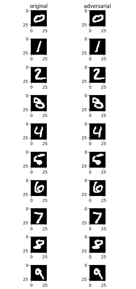
The following figure shows the effect before and after the attack. The left part is the original example, and the right part is the adversarial example generated after the untargeted FGSM attack. From a visual point of view, there is little difference between the right images and the left images, but all images on the right successfully mislead the model into misclassifying the sample as another incorrect categories.

adv_attack_result

Adversarial Defense

Natural Adversarial Defense (NAD) is a simple and effective adversarial example defense method, via adversarial training. It constructs adversarial examples during model training and mixes the adversarial examples with original examples to train the model. As the number of training iteration increases, the robustness of the model against adversarial examples improves. The NAD algorithm uses FGSM as the attack algorithm to construct adversarial examples.

Defense Implementation

Call the NAD API provided by MindArmour.

from mindspore.nn import SoftmaxCrossEntropyWithLogits
from mindarmour.defenses import NaturalAdversarialDefense


loss = SoftmaxCrossEntropyWithLogits(is_grad=False, sparse=False)
opt = nn.Momentum(net.trainable_params(), 0.01, 0.09)

nad = NaturalAdversarialDefense(net, loss_fn=loss, optimizer=opt,
                                bounds=(0.0, 1.0), eps=0.3)
net.set_train()
nad.batch_defense(np.concatenate(test_images), np.concatenate(test_labels),
                  batch_size=32, epochs=20)

# get accuracy of test data on defensed model
net.set_train(False)
acc_list = []
pred_logits_adv = []
for i in range(batch_num):
    batch_inputs = test_images[i]
    batch_labels = test_labels[i]
    logits = net(Tensor(batch_inputs)).asnumpy()
    pred_logits_adv.append(logits)
    label_pred = np.argmax(logits, axis=1)
    acc_list.append(np.mean(np.argmax(batch_labels, axis=1) == label_pred))
pred_logits_adv = np.concatenate(pred_logits_adv)
pred_logits_adv = softmax(pred_logits_adv, axis=1)

LOGGER.info(TAG, 'accuracy of TEST data on defensed model is : %s',
             np.mean(acc_list))
acc_list = []
for i in range(batch_num):
    batch_inputs = adv_data[i * batch_size: (i + 1) * batch_size]
    batch_labels = test_labels[i]
    logits = net(Tensor(batch_inputs)).asnumpy()
    label_pred = np.argmax(logits, axis=1)
    acc_list.append(np.mean(np.argmax(batch_labels, axis=1) == label_pred))

attack_evaluate = AttackEvaluate(np.concatenate(test_images),
                                 np.concatenate(test_labels),
                                 adv_data,
                                 pred_logits_adv)

LOGGER.info(TAG, 'accuracy of adv data on defensed model is : %s',
            np.mean(acc_list))
LOGGER.info(TAG, 'defense mis-classification rate of adversaries is : %s',
            attack_evaluate.mis_classification_rate())
LOGGER.info(TAG, 'The average confidence of adversarial class is : %s',
            attack_evaluate.avg_conf_adv_class())
LOGGER.info(TAG, 'The average confidence of true class is : %s',
            attack_evaluate.avg_conf_true_class())
LOGGER.info(TAG, 'The average distance (l0, l2, linf) between original '
            'samples and adversarial samples are: %s',
            attack_evaluate.avg_lp_distance())

Defense Effect

accuracy of TEST data on defensed model is : 0.973958
accuracy of adv data on defensed model is :  0.521835
defense mis-classification rate of adversaries is : 0.026042
The average confidence of adversarial class is : 0.67979
The average confidence of true class is : 0.19144624
The average distance (l0, l2, linf) between original samples and adversarial samples are: (1.544365, 0.439001, 0.300000)

After NAD is used to defend against adversarial examples, the model’s misclassification ratio of adversarial examples decreases from 95% to 48%, effectively defending against adversarial examples. In addition, the classification accuracy of the model for the original test dataset reaches 97%. The NAD function does not reduce the classification accuracy of the model.