Implementation of MindSpore-Powered Models in CV (2) — Fashion-MNIST Image Classification Experiment: Functional Programming

This experiment outlines the process of building a feedforward neural network (FNN) using MindSpore and leveraging the Fashion-MNIST dataset for model training and testing.

1. Objective

Master the construction of a basic FNN using MindSpore.

Learn how to use MindSpore to train simple image classification tasks.

Learn how to use MindSpore for testing and prediction in simple image classification tasks.

2. FNN Principles

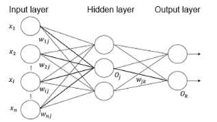
FNN is a type of artificial neural networks. It adopts a unidirectional multi-layer structure, in which each layer contains several neurons. In this neural network, every neuron is fed signals from a neuron in the preceding layer and generates output to the next layer. Layer 0 is called the input layer, the last layer is called the output layer, and other intermediate layers are called hidden layers. The network incorporates one or more hidden layers.

There is no feedback present throughout the network, with signals being transmitted in a unidirectional manner from the input layer to the output layer. The network can be depicted as a directed acyclic graph (DAG).

3. Experiment Environment

MindSpore 2.0 or later. The MindSpore version is updated periodically, and this guide will also be updated periodically to align with the version. This experiment can be conducted on the win_x86 and Linux OSs, and can run on CPUs, GPUs, and Ascend. If you run this experiment on a local computer, refer to the MindSpore Lab Environment Setup Manual to install MindSpore on the computer.

4. Data Processing

4.1 Dataset Preparation

Fashion-MNIST is an image dataset that serves as a replacement for the MNIST handwritten digit dataset. It is provided by the research department of Zalando, a Germany fashion technology company. It covers a total of 70,000 front images of different commodities from 10 classes. The size, format, and training/test dataset division of Fashion-MNIST are the same as those of the original MNIST dataset. The training/test dataset division is 60,000/10,000, and the images are 28 x 28 x 1 grayscale images.

Here is an introduction to the classic MNIST (handwritten digits) dataset. This classic dataset contains a large number of handwritten digits. For over a decade, researchers from the fields of machine learning, computer vision, artificial intelligence, and deep learning have used this dataset as one of the benchmarks for evaluating algorithms. The MNIST dataset has become one of the must-test datasets for algorithm developers. However, it is too simple. Many deep learning algorithms have achieved an accuracy of 99.6% on its test dataset.

Download the following four files from the Fashion-MNIST repository on GitHub to the local computer and decompress them:

train-images-idx3-ubyte training dataset images (47,042,560 bytes) train-labels-idx1-ubyte training dataset labels (61,440 bytes) t10k-images-idx3-ubyte test dataset images (7,843,840 bytes) t10k-labels-idx1-ubyte test dataset labels (12,288 bytes)

from download import download

#Download the MNIST dataset.
url = "https://ascend-professional-construction-dataset.obs.cn-north-4.myhuaweicloud.com:443/deep-learning/Fashion-MNIST.zip"
path = download(url, "./", kind="zip", replace=True)

4.2 Data Loading

Import MindSpore and auxiliary modules, which are described as follows:

MindSpore, used to build neural networks

NumPy, used to process certain data

Matplotlib, used to draw and display images

struct, used to process binary files

import os
import struct
from easydict import EasyDict as edict
import matplotlib.pyplot as plt
import numpy as np

import mindspore
import mindspore.dataset as ds
import mindspore.nn as nn
from mindspore.train import Model, Accuracy
from mindspore.train import ModelCheckpoint, CheckpointConfig, LossMonitor
from mindspore import Tensor

mindspore.set_context(mode=mindspore.GRAPH_MODE, device_target='Ascend')

Variable definitions:

cfg = edict({
    'train_size': 60000,    # training dataset size
    'test_size': 10000,     # test dataset size
    'channel': 1,           # number of image channels
    'image_height': 28,     # image height
    'image_width': 28,      # image width
    'batch_size': 60,
    'num_classes': 10,      # number of classes
    'lr': 0.001,            # learning rate
    'epoch_size': 10,       # number of training epochs
    # Change the path here to the actual path that stores your dataset. Use the train and test folders to store the training dataset and test dataset, respectively.
    'data_dir_train': os.path.join('./Fashion-MNIST/train/'),
    'data_dir_test': os.path.join('./Fashion-MNIST/test/'),
    'save_checkpoint_steps': 1,  # number of steps for saving a model
    'keep_checkpoint_max': 3,    # maximum number of models that can be saved
    'output_directory': './model_fashion',         # path for saving models
    'output_prefix': "checkpoint_fashion_forward"  # name of a saved model file
})

Read and process data. After being read by the data read function read_image, the data is in the following format:

Binary format of the images for training:

[offset] [type]          [value]          [description]
0000     32 bit integer  0x00000803(2051) magic number
0004     32 bit integer  60000            number of images
0008     32 bit integer  28               number of rows
0012     32 bit integer  28               number of columns
0016     unsigned byte   ??               pixel
0017     unsigned byte   ??               pixel
........
xxxx     unsigned byte   ??               pixel
Label format:
[offset] [type]          [value]          [description]
0000     32 bit integer  0x00000801(2049) magic number (MSB first)
0004     32 bit integer  60000            number of items
0008     unsigned byte   ??               label
0009     unsigned byte   ??               label
........
xxxx     unsigned byte   ??               label
The labels values are 0 to 9.
The code for reading data is as follows:
def read_image(file_name):
    file_handle = open(file_name, "rb")  # Open a document in binary mode.
    file_content = file_handle.read()    # Read data to the buffer.
    head = struct.unpack_from('>IIII', file_content, 0)  # Take the first four integers and return a tuple.
    offset = struct.calcsize('>IIII')
    imgNum = head[1]   # number of images
    width = head[2]    # width
    height = head[3]   # height
    bits = imgNum * width * height      # The data has 60,000 x 28 x 28 pixels.
    bitsString = '>' + str(bits) + 'B'  # fmt format: '>47040000B'
    imgs = struct.unpack_from(bitsString, file_content, offset)    # Take data and return a tuple.
    imgs_array = np.array(imgs).reshape((imgNum, width * height))  # Reshape the read data into a two-dimensional array of [number of images, image pixels].
    return imgs_array


def read_label(file_name):
    file_handle = open(file_name, "rb")  # Open a document in binary mode.
    file_content = file_handle.read()    # Read data to the buffer.
    head = struct.unpack_from('>II', file_content, 0)  # Take the first two integers and return a tuple.
    offset = struct.calcsize('>II')
    labelNum = head[1]  # number of labels
    bitsString = '>' + str(labelNum) + 'B'  # fmt format: '>47040000B'
    label = struct.unpack_from(bitsString, file_content, offset)  # Take data and return a tuple.
    return np.array(label)


def get_data():
    # Obtain files.
    train_image = os.path.join(cfg.data_dir_train, 'train-images-idx3-ubyte')
    test_image = os.path.join(cfg.data_dir_test, "t10k-images-idx3-ubyte")
    train_label = os.path.join(cfg.data_dir_train, "train-labels-idx1-ubyte")
    test_label = os.path.join(cfg.data_dir_test, "t10k-labels-idx1-ubyte")
    # Read data.
    train_x = read_image(train_image)
    test_x = read_image(test_image)
    train_y = read_label(train_label)
    test_y = read_label(test_label)
    return train_x, train_y, test_x, test_y

Data preprocessing and result image display

train_x, train_y, test_x, test_y = get_data()
# The first dimension is the batch size data, the second dimension is the number of image channels, and the third and fourth dimensions are the height and width.
train_x = train_x.reshape(-1, 1, cfg.image_height, cfg.image_width)
test_x = test_x.reshape(-1, 1, cfg.image_height, cfg.image_width)
# Normalize data to values between 0 and 1.
train_x = train_x / 255.0
test_x = test_x / 255.0
# Modify the data format.
train_x = train_x.astype('float32')
test_x = test_x.astype('float32')
train_y = train_y.astype('int32')
test_y = test_y.astype('int32')
print('number of samples in the training dataset: ', train_x.shape[0])
print('number of samples in the test dataset:', test_y.shape[0])
print('number of channels/image length/width: ', train_x.shape[1:])
# There are 10 classes, expressed in numbers from 0 to 9.
print('label style of an image: ', train_y[0])  

plt.figure()
plt.imshow(train_x[0,0,...])
plt.colorbar()
plt.grid(False)
plt.show()
Use the MindSpore GeneratorDataset API to convert data of the numpy.ndarray type into the dataset type.
# Convert the data to the dataset type.
XY_train = list(zip(train_x, train_y))
# Convert the data and label to the dataset type, and set the data to x and label to y.
ds_train = ds.GeneratorDataset(XY_train, ['x', 'y'])
ds_train = ds_train.shuffle(buffer_size=cfg.train_size).batch(cfg.batch_size, drop_remainder=True)
XY_test = list(zip(test_x, test_y))
ds_test = ds.GeneratorDataset(XY_test, ['x', 'y'])
ds_test = ds_test.shuffle(buffer_size=cfg.test_size).batch(cfg.batch_size, drop_remainder=True)

5. FNN Construction

The FNN is the simplest neural network architecture in which neurons are organized into layers, with each layer consisting of multiple neurons. Each neuron is connected only to a neuron at the previous layer. It receives an output of the previous layer as its input, and outputs the computation result to the next layer. The FNN is currently one of the most widely used and rapidly developing artificial neural networks. Layer 0 is called the input layer, the last layer is called the output layer, and other intermediate layers are called hidden layers. The network incorporates one or more hidden layers, which are formed by stacking fully connected layers.

# Define an FNN.
class Forward_fashion(nn.Cell):
    def __init__(self, num_class=10):  # a total of ten classes, with one image channel.
        super(Forward_fashion, self).__init__()
        self.num_class = num_class
        self.flatten = nn.Flatten()
        self.fc1 = nn.Dense(cfg.channel * cfg.image_height * cfg.image_width, 128)
        self.relu = nn.ReLU()
        self.fc2 = nn.Dense(128, self.num_class)

    def construct(self, x):
        x = self.flatten(x)
        x = self.fc1(x)
        x = self.relu(x)
        x = self.fc2(x)
        return x

6. Model Training

# Build a network.
network = Forward_fashion(cfg.num_classes)
# Define the loss function and optimizer of the model.
net_loss = nn.SoftmaxCrossEntropyWithLogits(sparse=True, reduction="mean")
net_opt = nn.Adam(network.trainable_params(), cfg.lr)
# Train the model.
model = Model(network, loss_fn=net_loss, optimizer=net_opt, metrics={"acc"})

# Define the train_loop function for training.
def train_loop(model, dataset, loss_fn, optimizer):
    # Define the forward propagation function.
    def forward_fn(data, label):
        logits = model(data)
        loss = loss_fn(logits, label)
        return loss

    # Define the differentiation function. Use mindspore.value_and_grad to obtain the grad_fn differentiation function, and output the loss and gradient.
    # Since taking derivatives with respect to model parameters is involved, set grad_position to None and pass trainable parameters.
    grad_fn = mindspore.value_and_grad(forward_fn, None, optimizer.parameters)

    # Define the one-step training function.
    def train_step(data, label):
        loss, grads = grad_fn(data, label)
        optimizer(grads)
        return loss

    size = dataset.get_dataset_size()
    model.set_train()
    for batch, (data, label) in enumerate(dataset.create_tuple_iterator()):
        loss = train_step(data, label)

        if batch % 100 == 0:
            loss, current = loss.asnumpy(), batch
            print(f"loss: {loss:>7f}  [{current:>3d}/{size:>3d}]")

# Define the test_loop function for testing.
def test_loop(model, dataset, loss_fn):
    num_batches = dataset.get_dataset_size()
    model.set_train(False)
    total, test_loss, correct = 0, 0, 0
    for data, label in dataset.create_tuple_iterator():
        pred = model(data)
        total += len(data)
        test_loss += loss_fn(pred, label).asnumpy()
        correct += (pred.argmax(1) == label).asnumpy().sum()
    test_loss /= num_batches
    correct /= total
    print(f"Test: \n Accuracy: {(100*correct):>0.1f}%, Avg loss: {test_loss:>8f} \n")

epochs = cfg.epoch_size
for t in range(epochs):
    print(f"Epoch {t+1}\n-------------------------------")
    train_loop(network, ds_train, net_loss, net_opt)
    test_loop(network, ds_test, net_loss)
print("Done!")

Use the Fashion-MNIST dataset to train the FNN model defined above.

7. Model Prediction and Visualization

# Use the test dataset to evaluate the model and print the overall accuracy.
metric = model.eval(ds_test)
print(metric)

class_names = ['T-shirt/top', 'Trouser', 'Pullover', 'Dress', 'Coat',
               'Sandal', 'Shirt', 'Sneaker', 'Bag', 'Ankle boot']

# Take a group of samples from the test dataset and input them to the model for prediction.
test_ = ds_test.create_dict_iterator().__next__()
# Use the key value to select samples.
test = Tensor(test_['x'], mindspore.float32)
predictions = model.predict(test)
softmax = nn.Softmax()
predictions = softmax(predictions)
predictions = predictions.asnumpy()
true_label = test_['y'].asnumpy()

for i in range(15):
    p_np = predictions[i, :]
    pre_label = np.argmax(p_np)
    print('' + str(i) + ' sample prediction result: ', class_names[pre_label], '   actual result: ', class_names[true_label[i]])

Visualize the prediction results.

Visualize the prediction results and input the prediction result sequence, real label sequence, and image sequence. The goal is to display the labels in red or blue based on the predicted values. Correct: blue label; incorrect: red label. Predict 15 images with labels and display the predicted results in a bar chart, with blue representing correct predictions and red representing incorrect predictions.

# -------------------Define the visualization function.--------------------------------
# Input the prediction result sequence, real label sequence, and image sequence.
# The goal is to display the labels in red or blue based on the predicted values. Correct: blue label; incorrect: red label.
def plot_image(predicted_label, true_label, img):
    plt.grid(False)
    plt.xticks([])
    plt.yticks([])
    # Display corresponding images.
    plt.imshow(img, cmap=plt.cm.binary)
    # Display the colors of the prediction results, with blue representing correct predictions and red representing incorrect predictions.
    if predicted_label == true_label:
        color = 'blue'
    else:
        color = 'red'
    # Display the formats and styles of corresponding labels.
    plt.xlabel('{},({})'.format(class_names[predicted_label],
                                    class_names[true_label]), color=color)
# Display the prediction results in a bar chart, with blue representing correct predictions and red representing incorrect predictions.
def plot_value_array(predicted_label, true_label,predicted_array):
    plt.grid(False)
    plt.xticks([])
    plt.yticks([])
    this_plot = plt.bar(range(10), predicted_array, color='#777777')
    plt.ylim([0, 1])
    this_plot[predicted_label].set_color('red')
    this_plot[true_label].set_color('blue')
# Predict 15 images with labels, and display the results.
num_rows = 5
num_cols = 3
num_images = num_rows * num_cols
plt.figure(figsize=(2 * 2 * num_cols, 2 * num_rows))

for i in range(num_images):
    plt.subplot(num_rows, 2 * num_cols, 2 * i + 1)
    pred_np_ = predictions[i, :]
    predicted_label = np.argmax(pred_np_)
    image_single = test_['x'][i, 0, ...].asnumpy()
    plot_image(predicted_label, true_label[i], image_single)
    plt.subplot(num_rows, 2 * num_cols, 2 * i + 2)
    plot_value_array(predicted_label, true_label[i], pred_np_)
plt.show()