Idea Sharing | MeshGPT Significantly Improves the Quality of 3D Geometry Representations

Background

Point clouds, voxels, and meshes are common 3D geometry representations. Compared to the former two, meshes provide more coherent surface representations. In addition, meshes are more controllable, easier to operate, more compact, and more suitable for downstream tasks.

However, current AI models extract meshes mainly through iso-surfacing, which results in dense triangular meshes to maintain the geometric details and topological features. Recently, a team at the Technical University of Munich published MeshGPT[1] that uses a decoder-only transformer to generate triangular meshes, making great progress in high-quality compact mesh generation.

1. Method

MeshGPT consists of two networks. The first is an encoder-decoder architecture that learns triangle embeddings through residual quantization. Then, a decoder-only GPT produces compact triangular meshes.

1.1 Learning Quantized Triangle Embeddings

As shown in Figure 1, the process of learning quantized triangle embeddings consists of four steps:

(1) A graph convolutional encoder converts the input mesh into rich features.

(2) The features are quantized into codebook embeddings using residual quantization, effectively reducing the sequence lengths and the pressure of the transformer.

(3) The embeddings are sequenced.

(4) A 1D ResNet decodes the embeddings to output simple 9-channel mesh embeddings. The input and output of the network are mesh information.

Now, let's look at the steps in detail, except the sequencing of embeddings.

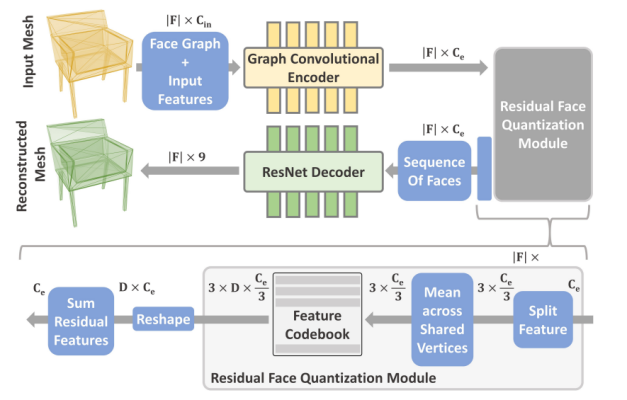
Figure 1 Learning quantized triangle embeddings

(1) GraphSAGE as the Encoder

The encoder used in MeshGPT is similar to PolyGen. PolyGen, if used directly, poses a challenge to the subsequent transformer training because it uses discrete coordinates as tokens, failing to capture geometric patterns due to the lack of information about neighboring meshes. Therefore, MeshGPT uses the graph neural network GraphSAGE[2] as the encoder. The core ideas of GraphSAGE are neighborhood sampling and feature aggregation.

Specifically, the SAGEConv layer of GraphSAGE performs linear transformation on the attribute features of a node and the sampled neighboring node features (by multiplying each with a W matrix and usually a ReLU activation function), connects the two, and then perform linear transformation again to obtain the feature representation of the target node, as shown in Figure 2. According to the practice of GraphSAGE, the number of sampling steps, k, does not need to be a large value. The effect is pretty good when k is 2, which means that sampling is extended to the 2-hop neighbors. In the GraphSAGE paper, S1·S2<=500. That is, the product of numbers of neighbors extended each time is less than 500, meaning that about 20 neighbors need to be extended each time.

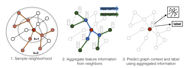
Figure 2 GraphSAGE visual illustration

The advantages of GraphSAGE are as follows: neighborhood sampling solves the out-of-memory problem of GCNs and is applicable to large graphs; inductive learning is used instead of transductive learning, eliminating the need for re-training based on node features and supporting incremental features; neighborhood sampling converts transductive nodes representing only one local structure into inductive node representation corresponding to multiple local structures, which effectively prevents overfitting and improves generalization.

In the paper, each mesh face can be considered as a node, and a face adjacent to the mesh face is connected to the mesh face itself through a non-directional line, as shown in Figure 3. Each node includes nine coordinate values (three vertices, each represented by three dimensional coordinates), the face normal, each angle of the face, and the area of the face. Then, the input mesh is converted into rich features through the SAGEConv layer mentioned above.

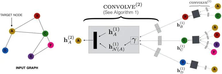
Figure 3 Application of the SAGEConv layer

(2) Residual Quantization

If the rich features generated in the previous step are directly used as embeddings, that is, a single code is used per face, the reconstruction accuracy is insufficient. Therefore, the paper refers to the residual vector quantization (RQ)[3] method and uses a stack of D (depth of RQ) codes per face.

RQ employs the idea of residual to convert the original one-layer codebook mapping into multi-layer mapping. It can be understood as that a shared codebook converts an original downsampled numerical matrix into a vector matrix with a depth of D. In this case, content corresponding to position (i,j) in each matrix becomes a D-dimensional vector, where each dimension represents a result of a residual layer. The advantages of the shared codebook (that is, the D layers share one codebook) are as follows: unlike separate codebooks that require extensive hyperparameter search for determining the codebook size of each depth, the shared codebook requires only the total codebook size to be determined; the shared codebook makes all code embeddings in each quantization depth available, so that the codes can be used at each depth for maximum utilization.

In the paper, the feature channel is decomposed into three mesh nodes on each face, and then features are aggregated through the shared mesh nodes. Each node retains D/3 codes, and finally D codes on each plane are obtained. This reduces computational cost and improves generation speed while ensuring reconstruction quality.

(3) 1D ResNet as the Decoder

The application of the decoder is simple. A 1D ResNet34 network is used as the decoder. Specifically, the paper finds that discrete prediction (for example, outputting the probability of each position given a set of discrete positions) tends to be better than predicting coordinates in a continuous real number domain.

1.2 Decoder-only GPT

The paper uses the GPT2-medium model, as shown in Figure 4. Its input is the embeddings of the SAGEConv output after RQ. The learned discrete positional encodings are used to indicate the sequence of mesh faces. In addition, it can be seen that the output mesh nodes are repeated (one node connects to multiple faces), so MeshLab is used to close the nodes.

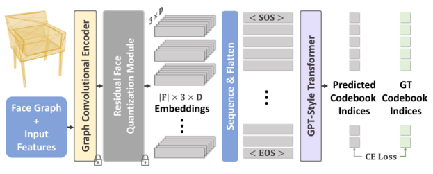
Figure 4 Decoder-only GPT used in the paper

2. Experiment Results

In the experiment of the paper, the encoder-decoder uses the RQ depth of 2, the corresponding D of each face is 6, and each face 192 dimensions. The codebook is updated using an exponentially weighted moving average (EWMA) of the features. The training is based on the ShapeNetV2 dataset and takes about two days using two GPUs. The context windows of the GPT2 model is 4608. The model is trained on four GPUs for about five days.

As shown in Figure 5, compared with other approaches, the proposed approach produces simplistic and compact meshes to represent 3D shapes with higher accuracy.

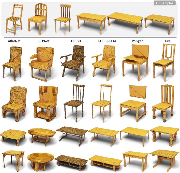
Figure 5 Comparison between the 3D mesh representation generated by the proposed approach and other approaches

3. Thoughts

The overall architecture in the paper is clear, and the accuracy and detail processing cost are greatly improved in 3D mesh representation. The overall idea of encoding meshes using GraphSAGE and performing RQ as well as some detail processing are worth learning. For example, compared with predicting coordinates in a continuous real number domain, discrete prediction usually performs better.

However, it should also be noted that the effect of the paper is based on intensive training on the four geometric types selected from the dataset. Therefore, the generalization of the network in the case of increased geometric types needs to be further investigated. At the same time, in the scientific computing scenario, it is necessary to consider how to establish a more direct and efficient matching between meshes representing 3D shapes and geometric discrete meshes in scientific computing.

References

[1] Siddiqui Y, Alliegro A, Artemov A, et al. MeshGPT: Generating Triangle Meshes with Decoder-Only Transformers[J]. arXiv preprint arXiv:2311.15475, 2023. https://arxiv.org/abs/2311.15475

[2] Hamilton W, Ying Z, Leskovec J. Inductive representation learning on large graphs[J]. Advances in neural information processing systems, 2017, 30.

[3] Doyup Lee, Chiheon Kim, Saehoon Kim, Minsu Cho, and Wook-Shin Han. Autoregressive image generation using residual quantization. In Proceedings of the IEEE/CVF Conference on Computer Vision and Pattern Recognition, pages 11523–11532, 2022.