Idea Sharing: GNN-MoM Graph Residual Learning EM Solver Based on MindSpore Elec

Background

MindSpore cooperates with Tsinghua University and Huawei Advanced Computing and Storage Laboratory to build an electromagnetic (EM) scattering algorithm for physics-informed graph residual learning, which achieves high accuracy in computing EM parameters of complex 3D targets.

Method of Moments (MoM) is a widely used numerical analysis method in EM computing. By solving the integral equations, MoM delivers excellent performance in EM scattering and radiation problems, and becomes popular in fields such as EM compatibility computation, antenna design, and microwave engineering. It is difficult to describe the meshes on 3D geometric surface in conventional EM computation, and matrix solving takes long and costs lots of computing resources. As an innovative neural network structure in machine learning, the Graph Neural Network (GNN) has been developing fast in recent years. Different from conventional deep learning models, GNNs can capture node relationships and network topologies. GNNs show great potential in fields such as drug discovery, recommendation systems, and natural language processing and become one of the hot topics of AI research.

With the development of AI technologies, the combination of GNNs and MoM is expected to solve the difficulty in geometric description and long duration of equation solving. Therefore, we construct a GNN-MoM solver[1] based on MindSpore Elec. The solver can apply MindSpore GNN operators to describe the shapes of complex 3D geometries, or utilize the automatic differentiation capability of MindSpore to construct the network mapping from the data residual to model updates. We accelerate the proposed GNN-MoM algorithm using GPU parallelism to achieve efficient modeling of EM scattering.

1. MoM Principle

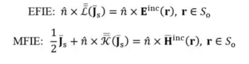
For perfect electric conductor (PEC) media, the equivalent surface current can be described by the electric-field integral equation (EFIE) and magnetic-field integral equation (MFIE):

Formula 1

_S_0 is the surface of the target. Einc, Hinc, and Js are respectively the incident current, magnetic field, and surface current. is the surface normal of the PEC target. In the EFIE, the second multiplier on the left of the equation can be written as:

Formula 2

_k_0 is the wavenumber. G(r,r') represents Green's function. In the MFIE, the second multiplier of the second term on the left of the equation can be expressed as:

Formula 3

To avoid interior resonances, the combined-field integral equation (CFIE) can be used, which is represented by a weighted combination of EFIE and MFIE and can be written as:

Formula 4

Z0 is the wave impedance. α is a value weighing EFIE and MFIE. Here, α is set to 0.5. By applying MoM and Rao–Wilton–Glisson (RWG) basis functions, CFIE can be discretized into a matrix equation, where u represents the unknown current coefficient vector, Z is the impedance matrix, and b is the excitation vector.

Formula 5

2. Physics-Informed Graph Residual Learning

Physics-informed supervised residual learning (PhiSRL) is proposed as a general deep learning framework for EM modeling[2]. PhiSRL uses deep neural networks (DNNs) to learn the update function of the unknown in the matrix equation through residuals and iteratively modify the unknown until convergence. In the framework of residual learning, the _k_th update equation during the iteration is as follows:

Formula 6

In 3D modeling, nonuniform discretization is usually used to represent arbitrary shapes. Compared with convolutional neural networks (CNNs), GNNs can better model such unstructured data. We construct a graph defined on the set of RWG basis functions of the 3D target. Each RWG basis function is considered a node in the graph. Edges in the graph are formed by connecting adjacent nodes. (Two nodes are adjacent if the corresponding RWG basis functions share a common endpoint.) The following figure shows the graph construction in the GNN-MoM algorithm.

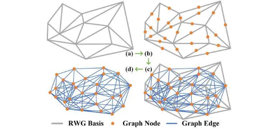
Figure 6

In residual learning–based 3D MoM EM modeling, we construct two GNNs with the same structure but different parameters. They learn the update rules of the real and imaginary parts of Uk separately. The _k_th update during equation solution can be written as:

Formula 7

The following figure describes the algorithm. During training, an unsupervised or supervised learning solution can be constructed using the automatic differentiation framework of MindSpore, so as to learn the iterative updates of unknown numbers in the GNN-MoM algorithm. Meanwhile, EM parameter computation of more complex 3D geometries can be solved through transfer learning.

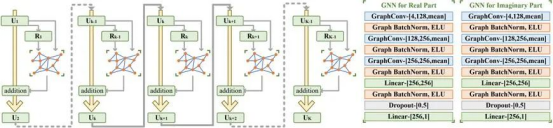
Figure 2

3. Experiments and Conclusions

3.1 Case 1: RCS Computation of Basic 3D PEC Targets

Radar Cross Section (RCS) measures the capability of a target object to reflect radar waves. The RCS size depends on the shape, size, material, and wavelength of the target. Accurate RCS computation and analysis are critical to the performance evaluation of the radar system and EM stealth.

With the MindSpore GNN code library, users can construct a GNN using discrete geometric meshes, describe the surface structures of complex 3D geometries, and complete multiple training modes such as supervised, unsupervised, and transfer learning through the automatic differential module.

Import the GNN code packages.

import os
import time
import numpy as np
import scipy.io as sio
import mindspore as ms
from mindspore import nn, ops
from mindspore.nn import optim
from mindspore.dataset import GeneratorDataset

During training, construct three different 3D geometries, use triangular meshes to discrete the 3D geometries, and use the GNN computing package of MindSpore to load the training dataset.

def process(self):
    ranidxmat = sio.loadmat(self.root + ';/randomidx.mat';)
    ranidx = ranidxmat['randomidx'][:][:].T
    for kk in range(int(self.totnum)):
        ii = ranidx[kk, 0]
        edgeneed = sio.loadmat('./GNN-CFIE-Dataset' + '/edgeneed' + str(ii) + '.mat')
        edgeidx = ms.Tensor((edgeneed['edgeidxfull'][:][:] / 1.0 - 1.0).astype(np.int32), ms.int32)
        edgeidxparnoself = ms.Tensor((edgeneed['edgeidxparnoself'][:][:] / 1.0 - 1.0).astype(np.int32), ms.int32)
        edgelabelR = ms.Tensor(edgeneed['edgelabelR'][:][:].astype(np.float32), ms.float32)
        edgelabelI = ms.Tensor(edgeneed['edgelabelI'][:][:].astype(np.float32), ms.float32)
        ZmatR = ms.Tensor(edgeneed['edgeZRfull'][:][:].astype(np.float32), ms.float32)
        ZmatI = ms.Tensor(edgeneed['edgeZIfull'][:][:].astype(np.float32), ms.float32)
        JmR = ms.Tensor(edgeneed['edgeJmR'][:][:].astype(np.float32), ms.float32)
        JmI = ms.Tensor(edgeneed['edgeJmI'][:][:].astype(np.float32), ms.float32)
        data = (edgeidx, edgelabelR, edgelabelI, ZmatR, ZmatI, JmR, JmI, JmR.shape[0], edgeidxparnoself)
        self.all_data.append(data)

Construct the loss computing class.

class LossCell(nn.Cell):
    def __init__(self, net, criterion):
        super().__init__()
        self.net = net
        self.criterion = criterion

    def construct(self, *args):
        netr, neti = self.net(*args[:-2])
        yr, yi = args[-2:]
        mseloss = (self.criterion(netr, yr) + self.criterion(neti, yi)) / 2
        return mseloss

Define a single-step training process, and iteratively update the network parameters with a proper optimizer.

model = GCNnet(channels)
criterion = nn.MSELoss()
loss_cell = LossCell(model, criterion)
exponential_decay_lr = nn.ExponentialDecayLR(learning_rate=0.001, decay_rate=0.9, decay_steps=25 * len(traindataset),
                                             is_stair=True)
optimizer = optim.Adam(loss_cell.trainable_params(), learning_rate=exponential_decay_lr)
train_cell = nn.TrainOneStepCell(loss_cell, optimizer)

end_epochs = 300

last_time = time.time()
start_time = last_time
for epoch in range(1, end_epochs + 1):
    noneedloss1 = model_train_epoch(epoch, traindataset, train_cell, criterion)
    now_time = time.time()
    print(f"epoch :{epoch}, loss_epoch: {noneedloss1}, time interval: {now_time - last_time}, "
          f"total_time: {now_time - start_time}")
    last_time = now_time
train_resloss.append(noneedloss1)

After the training is complete, select samples from the test dataset for inference. The result is as follows:

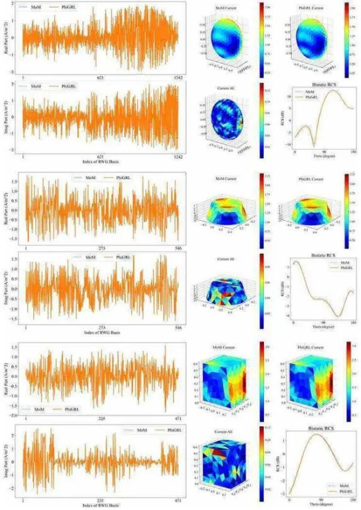
Figure 3

It can be seen that the RCSs computed by GNN-MoM and the RCSs computed by the conventional MoM are well fitted.

3.2 Case 2: RCS Computation of Complex 3D Geometries Based on Transfer Learning

In the MindSpore framework, the RCSs of complex 3D geometries, such as aircrafts, can be computed based on transfer learning. According to the GNN trained by basic 3D geometries, a small amount of RCS data of the aircraft-shape geometry is added. The following figure describes typical aircraft shapes.

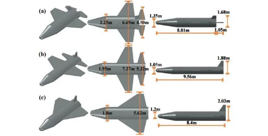
Figure 4

After the transfer learning is complete, perform inference on the aircraft dataset. The result is as follows:

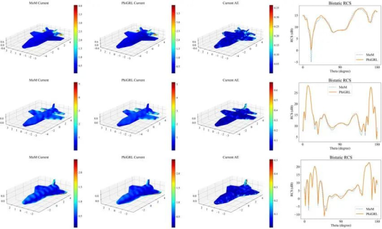
Figure 5

The surface currents and RCSs computed by GNN-MoM, and the surface current and RCSs predicted by GNN-MoM are in good agreement with the MoM results.

4. Summary and Outlook

We have launched a GNN-MoM EM solver based on MindSpore Elec, which can accurately describe the surface shapes of complex 3D geometries and quickly solve EM parameters such as surface current distribution and RCS, achieving the numerical accuracy equivalent to that of conventional MoM. We are expecting that more enterprises and research institutes can participate in the development and maintenance of the MindSpore Elec suite.

References

[1] T. Shan, et al., Solving Combined Field Integral Equations with Physics-informed Graph Residual Learning for EM Scattering of 3D PEC Targets [J], IEEE Transactions on Antennas and Propagation, 2023.

[2] T. Shan, et al., Physics-informed supervised residual learning for electromagnetic modeling [J], IEEE Transactions on Antennas and Propagation, 2023.

[3] R. Guo, et al., Physics embedded deep neural network for solving volume integral equation: 2d case [J], IEEE Transactions on Antennas and Propagation, 2021.