Idea Sharing: A Comprehensive Explanation on Fast Fourier Transform

Background

Discrete Fourier Transform (DFT) converts time-domain samples of signals into frequency-domain samples. It is the discrete version of Fourier transform in the time and frequency domains. The DFT is a crucial discrete transform mode utilized in numerous practical applications for conducting Fourier analysis. For example, in digital signal processing, sound pressure, radio signals, or daily temperatures can all be considered as samples of functions that vary with time and are collected within a finite time interval (window). In image processing, samples can be pixel values along rows or columns of a raster image. In mathematics, the DFT can be used to solve partial differential equations, convolution, or multiplication of large integers. In the AI4Science field, the DFT is also the basis of many algorithms, such as the Fourier Neural Operator (FNO).

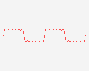
Figure 1 Fourier transform diagram

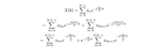
For a complex sequence with a given length N, the DFT is shown in formula 1, where x is the input sequence of N complex numbers, X is the corresponding output sequence, and the exponential power term is often referred to as a twiddle factor.

Formula 1

Formula 2

From formula 2, it can be seen that the DFT is essentially a vector matrix operation. Calculating the DFT of N points requires N^2 complex number multiplications and N(N–1) complex number additions, with a total time complexity of O(N^2×mul+N(N–1)×add).

Fast Fourier Transform (FFT) is a general term for efficient and fast calculation of the DFT or its inverse transform. The FFT utilizes the DFT features, such as symmetry and periodicity, to reduce repeated calculations in the DFT and lower the complexity. The introduction of the FFT algorithm has significantly expanded the applications of the DFT in engineering, science, mathematics, and other fields. It was selected as one of the top 10 algorithms in the 20th century by the IEEE Computing in Science & Engineering.

1. Methods

1.1 Cooley-Tukey Algorithm

The Cooley-Tukey algorithm is currently the most widely used and popular FFT algorithm. This method uses the divide-and-conquer strategy to recursively decompose the DFT of a sequence of length N into DFTs of two sub-sequences of length _N_1 and _N_2, respectively, as well as the complex number multiplication with the twiddle factor. Take the Cooley-Tukey algorithm whose radix is 2 as an example, where the length of N is a power of 2 (if not, padded with zeros), and decompose the DFT of a sequence of length N into DFTs of two sub-sequences of length N/2.

The Cooley-Tukey algorithm utilizes the symmetry and periodicity of the DFT to reduce repeated calculations in the DFT and lower the complexity. The derivation is as follows.

Formula 3

Therefore, the DFT of a sequence with N points is decomposed into DFTs of two sequences, each with N/2 points.

Formula 4

The signal flow is called a butterfly operation.

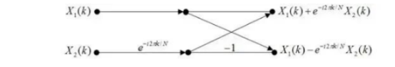
Figure 2 Butterfly operation units

It can be seen that each butterfly operation on the butterfly network requires one complex number multiplication and two complex number additions. For a sampling sequence x(n) (n = 8), the following butterfly network can be deduced.

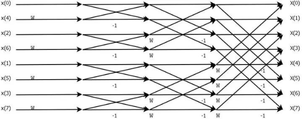
Figure 3 8-point butterfly network

According to the Cooley-Tukey algorithm process, assuming that a complex sequence of length N (= 2^L) is given with a radix of 2, a total of 2^(L-1) complex number multiplications and 2^L complex number additions are required. After recursion, the overall calculation complexity is O(N/2*logN×mul+NlogN×add), which is significantly lower than that of the DFT.

Furthermore, the Cooley-Tukey algorithm can also choose different radices as units to decompose sequences. Different decomposition methods produce FFT architectures with different layers. The larger the radix, the fewer the layers and complex multipliers, but the butterfly-shaped architecture of each level becomes more complex. Therefore, the common designs of architectures often have two, four and eight radices.

1.2 Split-radix Algorithm

The split-radix FFT algorithm (SRA) was proposed by Duhamel and Hollman in 1984. It is currently the FFT algorithm with the least number of multiplication and addition operations, and it has a good calculation structure and a shorter calculation program. The basic idea of the SRA algorithm is to use the radix-2 FFT algorithm for even sequences and the radix-4 FFT algorithm for odd sequences.

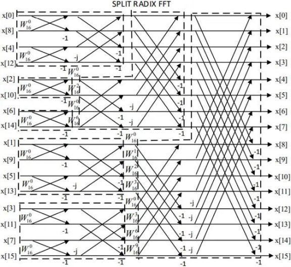
Figure 4 SRA algorithm diagram

1.3 Prime Factor Algorithm

The prime factor FFT algorithm (PFA), also known as the Good-Thomas algorithm, is also a type of fast Fourier transform. It decomposes the input DFT of size N into two-dimensional DFTs of sizes _N_1 and _N_2, where _N_1 and _N_2 are mutually prime. Then, the PFA can be recursively used or other FFT algorithms (such as Cooley-Tukey) can be chosen for calculation.

The PFA transforms the one-dimensional DFT problem into a multi-dimensional problem for calculation. The total time complexity is O(N(N_1+N_2)(mul+add)).

1.4 Rader's FFT Algorithm

The Rader algorithm is a fast algorithm for DFTs with prime inputs. It re-expresses the DFT of length N as a circular convolution of length N-1.

Formula 5

The circular convolution is also decomposable, and according to the convolution theorem, the N-1 circular convolution can be further decomposed into a smaller-scale DFT problem.

2. Conclusion

After learning the preceding FFT methods, we can summarize the following points:

2.1 The Organization of a Butterfly Network Will Affect the Entire Optimization

The butterfly network determines the data access pattern and butterfly computation execution sequence. Different implementations and optimizations of the same butterfly network may lead to different performance levels. For example, the PFA reduces the floating-point computing workload compared with the Cooley-Tukey algorithm. However, it requires more data accesses due to its complex mapping, making it more suitable for platform architectures where the data access overhead is less than the floating-point computation overhead.

2.2 The Performance of Butterfly Computation Will Directly Affect the Final Performance of FFT Algorithms

During the FFT calculation process, butterfly computation is repeatedly called. For example, based on the periodicity and symmetry of the DFT itself, common terms in the butterfly computation process can be exploited for repeated use at each level, which can reduce a significant amount of floating-point computation overhead.

2.3 Implementing High-Performance FFT Requires Integration with Hardware Architectures

For example, butterfly computation is independent of each other. SIMD can be used to process multiple butterfly computations in parallel, and the number of parallel computations depends on the situation of other components, such as the number of floating-point registers. Therefore, whether the hardware itself can be fully utilized directly affects the performance improvement of an FFT program.

3. Summary

With the development of heterogeneous computing frameworks, it has become very common to use compute units with different instruction sets and architectures to compose a computing system. Some researchers have shifted their focus from reducing the calculation overhead of FFT algorithms to implementing high-performance FFT algorithms on specific hardware architectures. There are already some mature high-performance FFT algorithm libraries in this area, such as FFTW, ARMPL, Intel MKL, Kunpeng's KML_FFT, AMD optimizing CPU libraries (AOCL), and CUDA fast Fourier transform library (CUFFT).

The Ascend heterogeneous computing architecture is leveraging its unique strengths to develop high-performance FFT libraries that enhance computing efficiency and reduce power consumption. We anticipate the release of these libraries in the near future.

References

[1] Cooley J W, Tukey J W. An algorithm for the machine calculation of complex Fourier series[J]. Mathematics of computation, 1965, 19(90): 297-301.

[2] Good I J. The interaction algorithm and practical Fourier analysis[J]. Journal of the Royal Statistical Society Series B: Statistical Methodology, 1958, 20(2): 361-372. https://doi.org/10.1111/j.2517-6161.1958.tb00300.x

[3] Thomas L H. Using a computer to solve problems in physics[J]. Applications of digital computers, 1963: 44-45.

[4] Duhamel P, Hollmann H. 'Split radix'FFT algorithm[J]. Electronics letters, 1984, 20(1): 14-16.

[5] Rader C M. Discrete Fourier transforms when the number of data samples is prime[J]. Proceedings of the IEEE, 1968, 56(6): 1107-1108. DOI: 10.1109/PROC.1968.6477

[6] Chen Tun, Li Zhihao, Jia Haipeng. Multi-Dimensional FFT implementation and optimization on ARM V8 platform[J]. Chinese Journal of Computers, 2019, 42(11): 2384-2402.

[7] Guo Jinxin, Zhang Guangting, Zhang Yunquan. High-Performance Implementation and Optimization of Cooley-Tukey FFT Algorithm[J]. Journal of Frontiers of Computer Science and Technology, 2022, 16 (6): 1304. DOI: 10.3778/j.issn.1673-9418.2011092