Idea Sharing | Analysis Overview of Replacing Traditional DFT and DeepH-E3 Models with Deep Learning Models
Idea Sharing | Analysis Overview of Replacing Traditional DFT and DeepH-E3 Models with Deep Learning Models
Author: Yu Fan Source: Zhihu
Background
In recent years, deep learning has contributed to significant progress in computational quantum chemistry. Existing deep learning methods demonstrated their efficiency and performance in various challenging quantum mechanics simulation tasks. As computing power today keeps increasing, deep learning is further combined with the first principle. Within the basic framework of physics, deep learning is integrated into equivariant neural networks (ENNs) on atomic and electronic scales to perform prediction in the quantum field. Especially in the field of the density functional theory (DFT), deep learning models, such as DeepH-E3 and QHNet, are developed based on ENNs to predict the Hamiltonian volume. This blog introduces the origin of the DFT, the principle of ENNs, a common ENN called e3nn, and finally the DeepH-E3 model, which is proposed by a research team of Tsinghua University to predict DFT Hamiltonian volume based on the E(3)-equivariant network [1].
1. DFT
DFT is a quantum mechanical method for studying electronic structures of multi-electron systems. Multi-electron systems are represented by the density functionals of electrons. DFT is widely used in physics and chemistry, especially for studying the properties of molecules and condensed matters.
Before the theory, system wave functions are calculated by solving the Schrödinger equation. As one of the basic equations in quantum mechanics, the form of the Schrödinger equation is as follows:
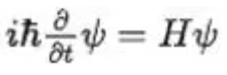
Formula 1: Time-dependent Schrödinger equation
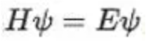
Formula 2: Time-independent Schrödinger equation
Ψ is a wave function that describes the state of microparticles. E represents kinetic energy. H represents Hamiltonian volume, which describes the evolution of quantum systems and can be expressed as the sum of kinetic and potential energy of particles.
For a multi-particle system containing N electrons and M atoms, the stationary Schrödinger equation corresponding to its Hamiltonian volume may be generally written as:

Formula 3: Schrödinger equation
The wave function has 3 x (M + N) variables, making the solution difficult.
DFT replaces the wave function with electron density to study the electronic structure of multi-electron systems. Density here is a function of three coordinates used to describe electron density, while a functional means that density is mapped to energy E as its function. DFT takes electron density as a base quantity and represents energy as a functional of electron density. Because electron density is only a function of spatial coordinates, which reduces the dimensions of a multi-electron system to 3, the solution of the Schrodinger equation is simplified.
In 1965, Walter Kohn and Lu Jeu Sham from University of California San Diego, proposed the Kohn-Sham (KS) equation. As the most common representative of the DFT, the KS equation transforms an interactive multi-particle system into a non-interactive single-particle system, and attributes the interaction between electrons to an unknown exchange-correlation potential.
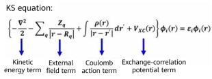
Formula 4: KS equation [4]
The exchange-correlation potential term refers to the energy difference between the interactive multi-particle system and non-interactive multi-particle system. In addition, the accurate function form of the term is unknown. Therefore, the term can only be represented as an approximate functional of electron density, for example, local-density approximation (LDA). Electron density is determined by the equation solution of the single-electron wave function described above. Therefore, the specific form of the equation depends on the solution itself and needs to be solved through self-consistent iteration.
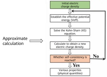
Figure 1 Approximate calculation process [4]
The calculation complexity is O (_N_3), where N is the number of electrons. The solution of large systems is still difficult.
2. Equivariant Network
When neural networks are used to calculate quantum properties, it is usually necessary to consider the impact of particle rotation on these properties. Some scalar values, such as energy values and distances between particles, are immune to the impact of particle rotation. Properties of some multi-dimensional vectors, such as values of force and Hamiltonian volume, need to be modified according to particle rotation, and such changes should be consistent from the beginning to the end of the network. Therefore, equivariant networks are commonly used for models related to the first principle.
2.1 What Is Equivariance?
Take a function as an example. If the transformation you apply to its input is also reflected on the output, the function is equivariant: f(g(x)) = g(f(x)).
2.2 What Is an ENN?
(1) Transformation done on the network input must be symmetrically mapped to the internal and output results.
(2) For example, for a three-dimensional atom structure, we need a neural network to predict its properties, including potential energy, number of electrons, and direction of force. If we rotate the atomic structure, its potential energy and number of electrons should remain unchanged because they are scalars; while the direction of the force on the structure should change accordingly because they are multi-dimensional vectors. The symmetric mapping must be reflected in the middle of the network and in the result. Therefore, an equivariant network is required to ensure the mapping.
2.3 Why Is Equivariance Needed?
To make a model symmetric, data augmentation is usually performed. For example, a two-dimensional animal image will be rotated by 10 different angles, and the results are fed to the neural network for training. However, for a three-dimensional model, for example, an atomic structure, augmentation is not that applicable. A simple three-dimensional model typically requires data augmentation of at least 500 rotations to cover properties of an atomic structure at different angles. But if an equivariant network is used, only one structure needs to be input.
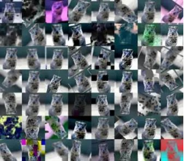
Figure 2 Two-dimensional animal images
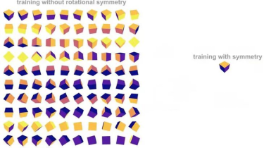
Figure 3 Three-dimensional model images [5]
3. e3nn: Spatial Transformer Neural Network Based on Three-Dimensional Euclidean Space
e3: spatial transformation group of three-dimensional Euclidean space, which can be divided into translation, rotation (SO(3) special orthogonal group), and inversion. Because the equivariance of translation is satisfied during convolution, we focus on rotation and inversion here: SO(3) × Z2 = O(3).
e3nn main concepts:
1. Group: spatial transformation type, for example, rotation and inversion.
2. Representation: defines a representation of a spatial transformation group to which the vector space belongs.
3. Irreducible representation (irreps): an indecomposable representation. Each irreps can be marked with (l, p). l is the order, which can be 0, 1, 2, and so on. p is parity, and p=e,o. The irreps of the l order is 2l + 1. For example, a vector with an order of 1 (that is, the dimension is 3) and odd parity can be briefly denoted as 1o.
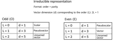
Figure 4 irreps introduction
As shown in the following figure, a1–a9 represent nine real numbers. If we regard a1–a3 as three scalars, a4–a6 a vector, and a7–a9 another vector, irreps of the matrix is represented as 3 × 0e + 2 × 1o. To rotate the matrix, perform different transformations based on different groups in irreps. As the values of the three scalars a1–a3 will not be affected by rotation, multiply their values by 1. While the two vectors a4–a6 and a7–a9 should be multiplied by corresponding rotation matrices.
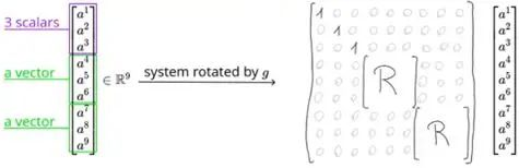
Figure 5 Example of rotation matrices [5]
The following describes how to decompose two multiplied irreps (how to decompose a tensor product).
 Formula 5: Decomposition of a tensor product For example: 2 ⊗ 1 = 1 ⊕ 2 ⊕ 3, 2 ⊗ 2 = 0 ⊕ 1 ⊕ 2 ⊕ 3. It is demonstrated that the reason why e3nn can maintain equivariance is that it determines the irreps of the network input, output, and intermediate results in advance. In this way, group transformation is performed according to the corresponding irreps, thereby preventing confusion. 4. DeepH-E3 DeepH-E3 is a general E{3} equivariant deep learning framework, which predicts the DFT Hamiltonian volume through a neural network with atomic structures {R} with spin orbits. DeepH-E3 can also be used for electronic predictions of larger material systems after training with DFT results of small material systems. The method is applicable to various material systems, such as general magic-angle twisted bilayer graphene (MATBG) or twisted van der Waals (vdW) materials, reducing the calculation cost by several orders of magnitude compared with using the DFT directly. The following figure shows the architecture of the entire network. {Zi} represents the atomic number, and |rij| represents the inter-atomic distance, which is used to construct a vector with an order equal to 0. ^rij represents the relative position between atoms, which is used to construct a vector with an order equal to 1 or 2. {Zi} is input to the elemental embedding module as the initial vertex. |rij| is input to the Gaussian bias as the edge feature. As the relative position between atoms, ^rij is input to a spherical harmonic function for mapping to generate Y(^rij). The spherical harmonic function Y^l maps a 3-dimensional vector to a vector of 2l + 1 dimensions, representing the coefficient when the input vector is decomposed into 2l + 1 basis spherical harmonic functions.
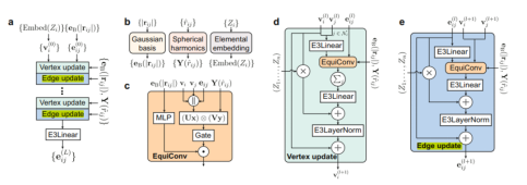
Figure 6 Overall structure of DeepH-E3 [1]
The generated vertex and edge features are updated for L times through blocks for vertex and edge update. The blocks encode the inter-atomic distance and relatively unknown information through equivariant convolution. The symbol "⋅" represents channel multiplication, and "||" represents vector concatenation.
Then, the message-passing method is used to obtain the information about the adjacent edges to update the vectors on edges and vertices.
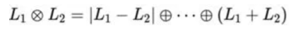
The final edge vector is passed to the Wigner-Eckart layer to display the DFT Hamiltonian volume. If spin-orbit coupling (SOC) is ignored, the output vector of the neural network is converted to the Hamiltonian volume through the Wigner Eckart layer according to the rule 1 ⊕ 2 ⊕ 3 = 1 ⊗ 2. If SOC is included, the output consists of two sets of real-number vectors, which are combined to form a complex-valued vector. These vectors are converted to spin-orbit DFT Hamiltonian volume according to another rule (1 ⊕ 2 ⊕ 3) ⊕ (0 ⊕ 1 ⊕ 2) ⊕ (1 ⊕ 2 ⊕ 3) ⊕ (2 ⊕ 3 ⊕ 4) = (1 ⊕ 1/2) ⊕ (2 ⊕ 1/2). ⊕ indicates tensor add, while ⊗ indicates tensor product.
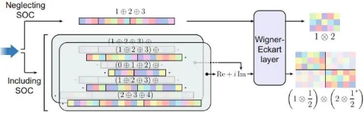
Figure 7 Wigner-Eckart layer [1]
5. Conclusion
This blog introduces the application of deep learning combined with the first principle, as well as the related physical basics. With the in-depth combination of deep learning and equivariant networks, more and more quantum features that are difficult to calculate using traditional methods can be predicted using neural networks. The trend helps research institutions study new materials, build material databases, and innovate applications.
References
[1]https://www.nature.com/articles/s41467-023-38468-8
[2]https://www.nature.com/articles/s43588-022-00265-6
[3]https://arxiv.org/abs/2207.09453
[4]https://www.bilibili.com/video/BV1vU4y1f7gQ/?spm\_id\_from=333.337.search-card.all.click