Idea Sharing: MindFlow-CFD, MindSpore-Based End-to-End Differentiable Solver

Author: Yu Fan | Source: Zhihu

Background

With the rapid development of AI technologies, the fusion of AI and computational fluid dynamics (CFD) has become an important branch of fluid mechanics. AI helps traditional CFD solvers break the precision and speed bottlenecks and improve computing efficiency.

Traditional CFD software, such as OpenFOAM and Fluent, provides comprehensive functions and excellent performance, as well as various extensions and secondary development interfaces for users to choose from. However, the interfaces of this type of software are not designed to easily integrate with AI models. Therefore, AI cannot be effectively used to optimize the training of the entire solution process.

In end-to-end deep learning, for a multi-phase data processing or learning system, the intermediate phases are replaced by a single neural network. CFD solvers are expected to have a similar feature that can optimize specific functions of the solvers based on the input flow field. An end-to-end differentiable CFD solver is developed based on an underlying AI framework to implement end-to-end training and inference. Existing differentiable CFD kits include PhiFlow, JaxCFD, and Jax-Fluids. PhiFlow supports NumPy, PyTorch, TensorFlow, and Jax backends and provides diversified solution, differentiation, and optimization functions. JaxCFD and Jax-Fluids are written in Jax. JaxCFD, released by Google, is mainly for turbulence time-domain and spectrum method solutions and can accelerate simulation using multiple AI models. Jax-Fluids, written by Professor Adams' team at the Technical University of Munich, provides rich numerical formats and turbulence models for compressible two-phase flows.

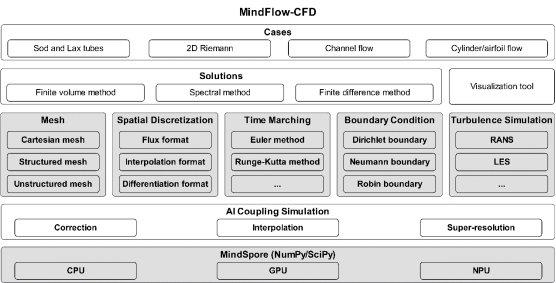
MindFlow is a fluid simulation suite developed based on MindSpore. It supports AI flow field simulation in industries such as aerospace, ship manufacturing, and energy and electricity. Based on MindSpore and MindFlow, we developed MindFlow-CFD, an end-to-end differentiable fluid solver, to provide efficient and easy-to-use AI computing fluid simulation software for scientific research personnel in the industry and college teachers and students, implementing joint development, research, and exploration of differentiable CFD.

The following figure shows the overall MindFlow-CFD planning, which aims to provide an end-to-end differentiable solution suite for viscous compressible flows. To improve solution efficiency, we use the JIT acceleration feature of MindSpore to compile the solution of each step to a computational graph and perform simulation by combining dynamic and static graphs. In this way, the simulation efficiency is improved. The code of MindFlow-CFD has been released on Gitee.

https://gitee.com/mindspore/mindscience/tree/master/MindFlow

Now, let's use a case to show the MindFlow-CFD solution process.

Case 1: Couette Flow

Couette flow is one of the most basic flows in fluid mechanics. Using MindFlow-CFD, you can build a CFD simulation process based on your programming habits.

simulator = Simulator(config)

runtime = RunTime(config['runtime'], simulator.mesh_info, simulator.material)

Simulator and Runtime are high-level APIs of MindFlow-CFD and are used to perform simulation and control simulation time.

mesh_x, mesh_y, _ = simulator.mesh_info.mesh_xyz()

pri_var = couette_ic_2d(mesh_x, mesh_y)

con_var = cfd.cal_con_var(pri_var, simulator.material)

The grid coordinates are directly obtained by simulator, and a corresponding initial condition may be directly calculated according to the grid coordinates. The primitive physical variable pri_var needs to be converted into a conservative variable con_var for solution.

The code of the solution process is as follows. The iteration of the conservative variable is performed in integration_step of simulator. The Runge-Kutta method is used to integrate the right part of the equation to solve the flow field of the next time step. In addition, runtime controls the time step and time advance.

while runtime.time_loop(pri_var):

runtime.compute_timestep(pri_var)

con_var= simulator.integration_step(con_var, runtime.timestep)

pri_var = cfd.cal_pri_var(con_var, simulator.material)

runtime.advance()

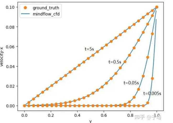
The following figure shows the final iteration result. The speed distribution in the x direction at different moments is shown in the figure, which is consistent with the related theories.

out_channels=nn_config['net']['out_channels'],

layers=nn_config['net']['layers'],

neurons=nn_config['net']['neurons'],

residual=False,

act="tanh")

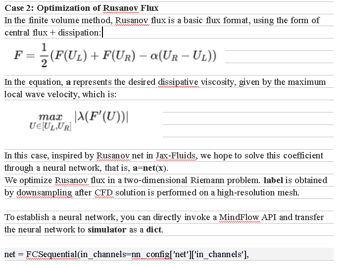
net_dict = {'rusanov_net': net}

simulator = Simulator(nn_config, net_dict)

The training process uses functional programming. MindFlow-CFD is end-to-end differentiable. Therefore, the solution process can be directly written in the forward function.

def advance(pri_var):

con_var = cal_con_var(pri_var, simulator.material)

for _ in range(1):

con_var = simulator.integration_step(con_var, runtime.timestep)

pri_var = cal_pri_var(con_var, simulator.material)

return pri_var

It should be noted that in the solver, calculation is performed on only one working condition. However, in AI model training, to improve training efficiency, many working conditions need to be trained in one batch. To meet this requirement, we can use the new function provided by MindSpore 2.0, that is, vmap automatic vectorization, to add a batch dimension to the input and output of the forward function.

batch_adv = ops.vmap(advance, in_axes=0, out_axes=0)

Finally, grad_fn can be used to implement loss, reverse derivation, and training. These steps are the same as those for training a neural network through functional programming.

def forward_fn(x, label):

predict = batch_adv(x)

loss = loss_fn(predict, label, x)

return loss

grad_fn = ops.value_and_grad(forward_fn, None, optimizer.parameters, has_aux=False)

@jit

def train_step(inputs, labels):

loss, grads = grad_fn(inputs, labels)

loss = ops.depend(loss, optimizer(grads))

return loss, grads

for i in range(train_config['epochs']):

net.set_train()

for j, item in enumerate(train_iterator):

u0 = item['u0']

ut = item['ut']

loss, grads = train_step(u0, ut)

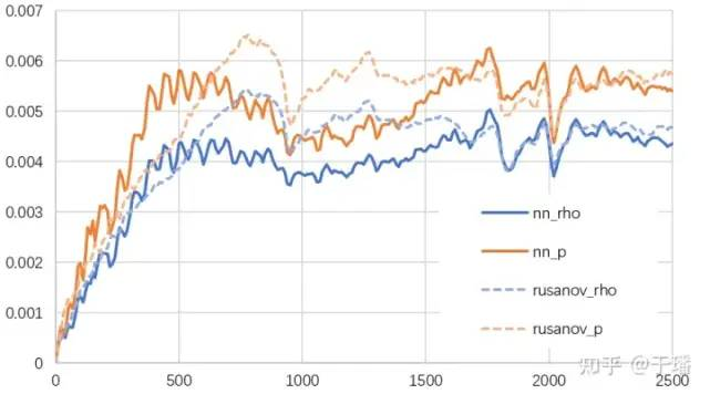
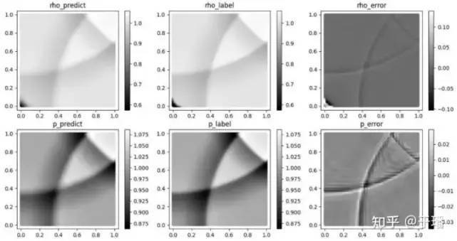
The training uses the data of the first 1000 time steps to infer the flow field changes of the entire 2500 time steps. The following figure shows the relative L1loss of density and pressure. Compared with the traditional Rusanov flux, the relative error of fusion calculation is smaller and more stable in long-term predictions.

Conclusion

In this blog post, we investigated the bottlenecks of traditional CFD solvers and the research trend of the fusion of AI and CFD computing, and summarized the status of end-to-end differentiable CFD solvers. We then tried the MindFlow-CFD solver, which can implement differentiable solution of compressible flows and integrate AI models to implement end-to-end optimization. In addition to supporting traditional methods, MindFlow-CFD makes it possible for AI fusion fluid calculation.

The fusion of AI and CFD computing is an emerging research paradigm of CFD and has potential in computing acceleration, turbulence model, and combustion model.

For more cases, see:

https://gitee.com/mindspore/mindscience/tree/master/MindFlow