MindSpore Learning and Practice | How Gradient Accumulation Helps with Limited Training Memory

Background

Out of memory (OOM) is an often undesired state of computer operation where no additional memory can be allocated for use by programs or the operating system. As shown in the figure below, if the requested memory of a model exceeds the actual device memory size, an "Out of Memory" error will occur. In general, setting the batch size to a large value or having a small amount of memory on the compute device (such as GPU and NPU) often triggers this error.

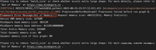
Error reported when the memory of MindSpore is insufficient on Ascend

When faced with this issue, developers often resort to decreasing the batch sizes. However, this may not be a viable solution as many models are already quite large, especially with the widespread use of pre-trained models. For instance, when I was fine-tuning a BERT model in 2019 using a single 1080Ti with 11 GB memory, the maximum batch size I could set was only 4. But batch size is a hyperparameter that greatly affects the training performance, and in many cases, good results can only be achieved by using the values obtained by developers' original tuning. At this point, if you have the budget, you can add more cards; otherwise you can only find another way to optimize your computing card with limited memory.

Gradient Accumulation

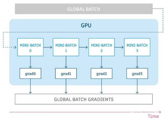
Gradient accumulation, as the name suggests, is to accumulate gradient values obtained from multiple computations, and then update parameters at a time. As shown in the figure below, assuming we have a global batch with a size of 256, when the single-card training memory is insufficient, we divide the global batch into four mini-batches with a size of 64 each. Then, send one mini-batch to obtain a gradient at each step, and accumulate the gradients obtained multiple times before updating the parameters. This can simulate the training effect of using only a single global batch.

Simply put, this is trading time for space. By extending the training time, we can train a large batch on small devices.

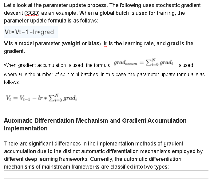
1. Tensor-centered automatic differentiation: We can configure the requires_grad parameter for tensors to determine whether to use gradients. Each tensor object has the grad_fn attribute to store reverse operations involved in the tensor and the grad attribute to store the gradient of the tensor. The gradient is obtained by computing the loss.backward() scalar. Most frameworks in the industry, such as PyTorch, Paddle, OneFlow, and MegEngine, use this mechanism because the API usage is highly consistent with the backpropagation mode.

2. Functional automatic differentiation: This mechanism treats the forward propagation of neural networks as the input to the loss function, obtains the backward propagation function through function transformation, and calls the backward propagation function to obtain the gradient. Jax and MindSpore frameworks use this mechanism. In addition, GradientTape of TensorFlow can be regarded as a variant of this mechanism.

The principles of automatic differentiation are consistent between these two mechanisms, with the core difference being whether or not they expose the bottom-layer APIs of automatic differentiation. Frameworks such as PyTorch are more focused on pure deep learning, and therefore only emphasize the use of backward, which is well-suited to the usage habits of their target users. Jax and MindSpore are positioned as frameworks focusing more on bottom layers, with Jax explicitly stating that it is a numerical compute framework, and MindSpore positioning itself as an AI + scientific compute framework. Therefore, a functional automatic differentiation design is more in line with the positioning of these frameworks.

The following uses MindSpore as an example to describe the implementation of gradient accumulation.

Implementation in MindSpore

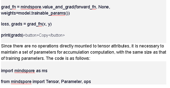
For functional automatic differentiation, because bottom-layer APIs are exposed, the gradients are directly calculated and returned. The following is a simple example:

@ms.jit_class
class Accumulator():
    def __init__(self, optimizer, accumulate_step):
        self.optimizer = optimizer
        self.inner_grads = optimizer.parameters.clone(prefix="accumulate_", init='zeros')
        self.zeros = optimizer.parameters.clone(prefix="zeros_", init='zeros')
        self.counter = Parameter(Tensor(1, ms.int32), 'counter_')
        assert accumulate_step > 0
        self.accumulate_step = accumulate_step
        self.map = ops.HyperMap()

    def __call__(self, grads):
        # Accumulate the gradient obtained in each step to inner_grads of the accumulator.
        self.map(ops.partial(ops.assign_add), self.inner_grads, grads)
        if self.counter % self.accumulate_step == 0:
            # If the target number of steps for accumulation is reached, optimize and update the parameters.
            self.optimizer(self.inner_grads)
            # Clear inner_grads after the parameter optimization and update.
            self.map(ops.partial(ops.assign), self.inner_grads, self.zeros)
        # Add one computation step.
        ops.assign_add(self.counter, Tensor(1, ms.int32))

        return True

The preceding code implements an independent accumulator, where self.inner_grads is the parameter for separately storing accumulated gradients. You only need to clone a set of training parameters. A counter also needs to be independently maintained to ensure that parameters are updated at an interval specified by accumulate_step.

The implementation steps in the __call__ function are the same as those in PyTorch, both involve continuous accumulation of gradients, parameter update after the target number of steps is reached, and gradient clearance. As an accumulator is maintained independently, here the optimizer is used as an input parameter for computation in the accumulator. The complete training process is as follows:

accumulate_step = 2

loss_fn = nn.CrossEntropyLoss()
optimizer = nn.SGD(model.trainable_params(), 1e-2)
accumulator = Accumulator(optimizer, accumulate_step)

def forward_fn(data, label):
    logits = model(data)
    loss = loss_fn(logits, label)
    # Divide loss by accumulate_step.
    return loss / accumulate_step

grad_fn = value_and_grad(forward_fn, None, model.trainable_params())

@ms.jit
def train_step(data, label):
    loss, grads = grad_fn(data, label)
    loss = ops.depend(loss, accumulator(grads))
    return loss

Because APIs of functional automatic differentiation lie in bottom layers, the handling of gradients can be more flexible. You can cancel the mean operation from forward_fn and change self.optimizer(self.inner_grads) to self.optimizer(self.map(ops.div, self.inner_grads, self.accumulate_step)) in the accumulator to achieve the same effect.

Additionally, you can determine whether to execute the optimizer separately from the accumulator, allowing the accumulator to purely handle accumulation and clearing operations, according to your usage habits. This is the flexibility advantage of bottom-layer APIs, but correspondingly, compared to PyTorch which encapsulates most operations, using bottom-layer APIs is more complex, and is more suitable for principle learning.