Idea Sharing: AD_FDTD, MindSpore-Based Device-to-Device Differential Electromagnetic Solver

Background

MindSpore and Huawei Noah's Ark Laboratory have jointly built a device-to-device differential electromagnetic solver of finite-difference time-domain (FDTD), whose performance has been verified in products such as patch antennas, patch filters, and 2D inverse electromagnetic scattering.

Proposed by K.S.Yee in 1966, FDTD performs discrete and iterative calculation on the E-field and H-field of an electromagnetic field by alternative sampling in space and time. After more than five decades of development, FDTD has become a well-established numerical method. It is widely used in various scenarios, including the analysis of radiation antennas, research on microwave devices and waveguide structures, cross-sectional calculation of scattering and radar, analysis of periodic structures, electronics packaging, and propagation and scattering of nuclear electromagnetic pulses. Nonetheless, traditional numerical methods still face challenges like low computation efficiency and complex computation process, especially in inverse electromagnetic waves.

With the development of AI technologies, AI converged computing (integration of AI and traditional numerical methods) is expected to solve the preceding problems. With this context, we've constructed a device-to-device differential electromagnetic solver AD_FDTD based on MindSpore. This solver is able to rewrite an FDTD forward solution process using MindSpore's neural network operators. It can also optimize medium parameters for inverse electromagnetic waves using MindSpore's automatic differentiation capability. In the future, it is anticipated that some complex solution processes in FDTD will be replaced by AI agent models. Device-to-device differential electromagnetic solvers provide more exploration and development possibilities for electromagnetic technologies.

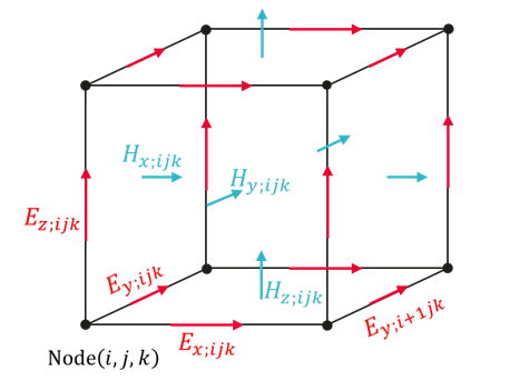
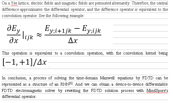
1. Principle of Differential FDTD Solver

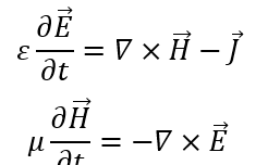
The time-domain Maxwell equations can be presented in the following formats:

Numerical solution requires us to discretize the equations by processing partial time derivatives first. FDTD alternately updates electric fields and magnetic fields in a leapfrog manner, which generates the following time-stepping formats:

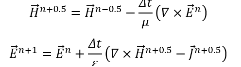
A process of updating electromagnetic fields according to the foregoing formulas can be seen as a recurrent neural network (RNN).

2. Application Cases

This part describes features and usage of the solver through cases of forward simulation and reverse optimization.

Case: https://www.mindspore.cn/mindelec/docs/en/master/AD_FDTD.html

Code: https://gitee.com/mindspore/mindscience/tree/master/MindElec/examples/AD_FDTD

2.1 Forward Simulation: S-parameter Simulation of a Patch Antenna

Electromagnetic simulation is widely used in the product design processes of antennas, chips, and mobile phones. The goal is to obtain the transmission characteristics (such as scattering parameters and electromagnetic fields) of the target to be simulated. The scattering parameters (S-parameters) are network parameters based on the input wave and the reflected wave, and are used to analyze microwave circuits.

By using APIs provided by the code package, you can establish the S-parameter simulation process as follows.

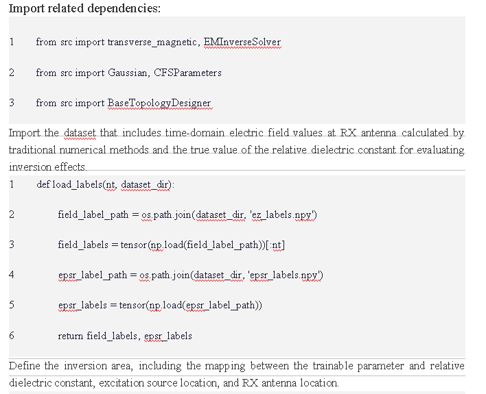
Import related dependencies:

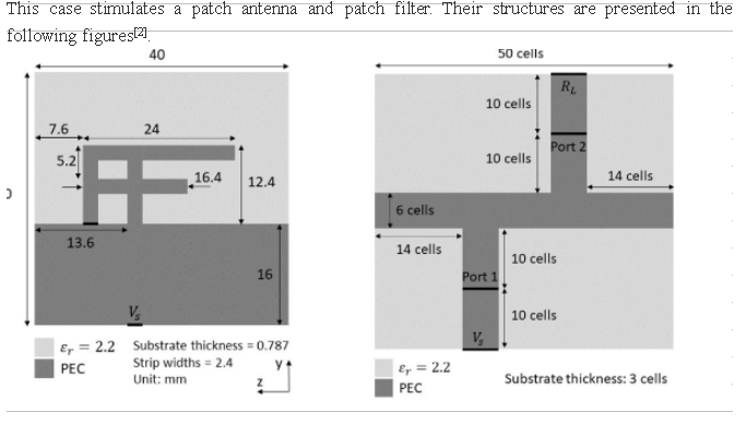
Define the antenna structure using APIs provided by the code packaged based on the antenna design diagram:

Patch antenna:

1    def get_invert_f_antenna(air_buffers, npml):
2        """ Get grid for IFA. """
3        # Define FDTD grid
4        cell_lengths = (0.262e-3, 0.4e-3, 0.4e-3)
5        obj_lengths = (0.787e-3, 40e-3, 40e-3)
6        cell_numbers = (
7            2 * npml + 2 * air_buffers[0] + int(obj_lengths[0] / cell_lengths[0]),
8            2 * npml + 2 * air_buffers[1] + int(obj_lengths[1] / cell_lengths[1]),
9            2 * npml + 2 * air_buffers[2] + int(obj_lengths[2] / cell_lengths[2]),
10        )
11        grid = GridHelper(cell_numbers, cell_lengths, origin=(
12            npml + air_buffers[0] + int(obj_lengths[0] / cell_lengths[0]),
13            npml + air_buffers[1],
14            npml + air_buffers[2],
15        ))
16        # Define antenna
17        grid[-3:0, 0:100, 0:100] = UniformBrick(epsr=2.2)
18        grid[0, 0:71, 60:66] = PECPlate('x')
19        grid[0, 40:71, 75:81] = PECPlate('x')
20        grid[0, 65:71, 21:81] = PECPlate('x')
21        grid[0, 52:58, 40:81] = PECPlate('x')
22        grid[-3:0, 40, 75:81] = PECPlate('y')
23        grid[-3, 0:40, 0:100] = PECPlate('x')
24        # Define sources
25        grid[-3:0, 0, 60:66] = VoltageSource(amplitude=1., r=50., polarization='xp')
26        # Define monitors
27        grid[-3:0, 0, 61:66] = VoltageMonitor('xp')
28        grid[-1, 0, 60:66] = CurrentMonitor('xp')
29        return grid

Patch filter:

1    def get_microstrip_filter(air_buffers, npml):
2        """ microstrip filter """
3        # Define FDTD grid
4        cell_lengths = (0.4064e-3, 0.4233e-3, 0.265e-3)
5        obj_lengths = (50 * cell_lengths[0],
6                       46 * cell_lengths[1],
7                       3 * cell_lengths[2])
8        cell_numbers = (
9            2 * npml + 2 * air_buffers[0] + int(obj_lengths[0] / cell_lengths[0]),
10            2 * npml + 2 * air_buffers[1] + int(obj_lengths[1] / cell_lengths[1]),
11            2 * npml + 2 * air_buffers[2] + int(obj_lengths[2] / cell_lengths[2]),
12        )
13        grid = GridHelper(cell_numbers, cell_lengths, origin=(
14            npml + air_buffers[0],
15            npml + air_buffers[1],
16            npml + air_buffers[2],
17        ))
18        # Define antenna
19        grid[0:50, 0:46, 0:3] = UniformBrick(epsr=2.2)
20        grid[14:20, 0:20, 3] = PECPlate('z')
21        grid[30:36, 26:46, 3] = PECPlate('z')
22        grid[0:50, 20:26, 3] = PECPlate('z')
23        grid[0:50, 0:46, 0] = PECPlate('z')
24        # Define sources
25        grid[14:20, 0, 0:3] = VoltageSource(1., 50., 'zp')
26        # Define load
27        grid[30:36, 46, 0:3] = Resistor(50., 'z')
28        # Define monitors
29        grid[14:20, 10, 0:3] = VoltageMonitor('zp')
30        grid[14:20, 10, 3] = CurrentMonitor('yp')
31        grid[30:36, 36, 0:3] = VoltageMonitor('zp')
32        grid[30:36, 36, 3] = CurrentMonitor('yn')
33        return grid

Define an S-parameter solver based on differential FDTD and find the solution:

1        # define fdtd network
2        fdtd_net = full3d.ADFDTD(grid_helper.cell_numbers, grid_helper.cell_lengths,
3                                    nt, dt, ns, antenna, cpml)
4        # define solver
5        solver = SParameterSolver(fdtd_net)
6        # solve
7        outputs = solver.solve(waveform_t)

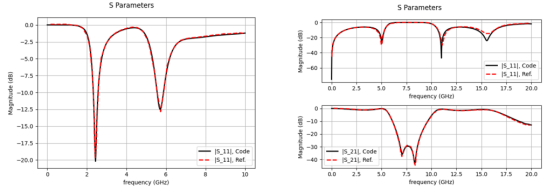
The comparison of the S-parameter calculated by differential FDTD between the referenced paper[1] indicates that the accuracy of calculation results produced by differential FDTD is equivalent to those of traditional numerical algorithms.

2.2 Reverse Optimization: Solving Electromagnetic Inverse Scattering

This case describes how to use MindSpore's automatic differential capability to reconstruct a dielectric based on the time-domain signals received by the receive antenna using the differential FDTD method. This case solves the electromagnetic inverse scattering in two-dimensional mode[3].

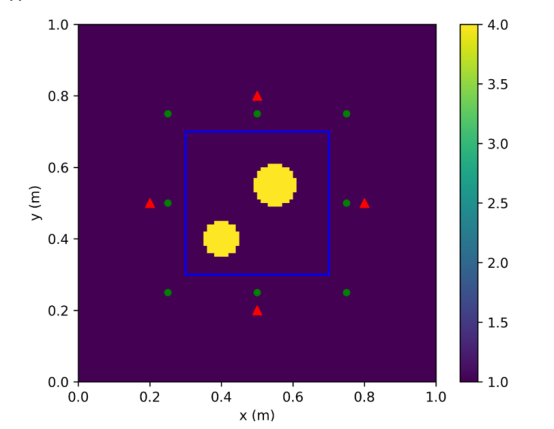
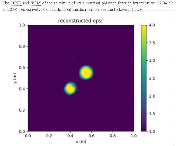
The entire simulation area is divided into 100 x 100 grids, and the 40 x 40 grids (blue square) are used as the optimization area. Four excitation sources (red triangles) and eight observation points (green dots) are set outside the optimization area. The inversion targets are two dielectrics with relative dielectric constant being 4.

By using APIs provided by the code package, you can establish a complete optimization process for electromagnetic inverse scattering as follows.

1    class InverseDomain(BaseTopologyDesigner):
2        def generate_object(self, rho):
3            """Generate material tensors.
4            """
5            # generate background material tensors
6            epsr = self.background_epsr * self.grid
7            sige = self.background_sige * self.grid
8            epsr[30:70, 30:70] = self.background_epsr + elu(rho, alpha=1e-2)
9            return epsr, sige
10    
11        def update_sources(self, *args):
12            """Set locations of sources.
13            """
14            sources, _, waveform, _ = args
15            jz = sources[0]
16            jz[0, :, 20, 50] = waveform
17            jz[1, :, 50, 20] = waveform
18            jz[2, :, 80, 50] = waveform
19            jz[3, :, 50, 80] = waveform
20            return jz
21    
22        def get_outputs_at_each_step(self, *args):
23            """Compute output each step.
24            """
25            ez, _, _ = args[0]
26            rx = [
27                ez[:, 0, 25, 25],
28                ez[:, 0, 25, 50],
29                ez[:, 0, 25, 75],
30                ez[:, 0, 50, 25],
31                ez[:, 0, 50, 75],
32                ez[:, 0, 75, 25],
33                ez[:, 0, 75, 50],
34                ez[:, 0, 75, 75],
35            ]
36            return vstack(rx)

The elu activation function is used to guarantee that no unphysical dielectric constant will appear during the solution.

Define a differential FDTD network. As mentioned before, a process of solving the time-domain Maxwell equations by FDTD can be seen as an RNN. In this case, the update process of each field in an FDTD solving process of the 2D TM mode is as follows.

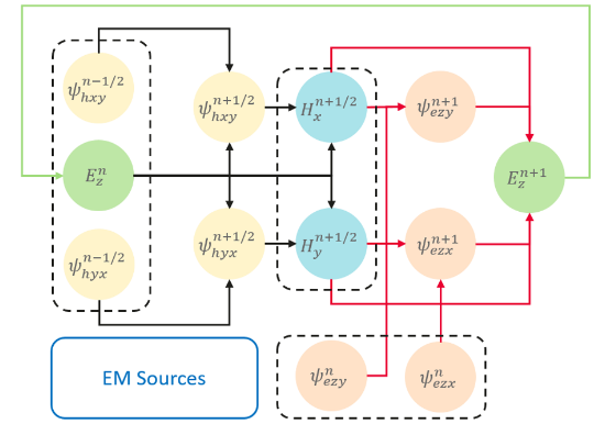
The preceding update process has been implemented in the code. You can directly invoke related APIs to define a differential FDTD network.

Define the loss function and optimizer for training and evaluation:

1    # define fdtd network
2    fdtd_net = transverse_magnetic.ADFDTD(
3        cell_numbers, cell_lengths, nt, dt, ns,
4        inverse_domain, cpml, rho_init)
5    # define solver for inverse problem
6    epochs = options.epochs
7    lr = options.lr
8    loss_fn = nn.MSELoss(reduction='sum')
9    optimizer = nn.Adam(fdtd_net.trainable_params(), learning_rate=lr)
10   solver = EMInverseSolver(fdtd_net, loss_fn, optimizer)
11   # solve
12   solver.solve(epochs, waveform_t, field_labels)

3. Summary

This MindSpore-based device-to-device electromagnetic solver of differential FDTD is capable of implementing differentiable solutions for electromagnetic simulation. Its effectiveness has been successfully demonstrated in scenarios such as patch antennas, patch filters, and 2D electromagnetic inverse scattering. In the case of the patch antenna and patch filter, the simulation accuracy of S-parameter is equivalent to that produced by traditional numerical methods. In the case of 2D electromagnetic inverse scattering, the structural similarity (SSIM) of dielectric parameters obtained through inversion reaches 96%. Enterprises and research institutes are welcomed to participate in our open source community to continuously evolve differential FDTD electromagnetic solvers and jointly explore the future of AI-driven electromagnetism.

References

[1] L. Guo, et al., Electromagnetic Modeling Using an FDTD-Equivalent Recurrent Convolution Neural Network: Accurate Computing on a Deep Learning Framework [J], IEEE Antennas and Propagation Magazine, 2021.

[2] A. Z. Elsherbeni and V. Demir, The Finite-Difference Time-Domain Method for Electromagnetics with MATLAB Simulations [M], 2ed, 2016.

[3] P. Zhang, et al., A Maxwell's Equations Based Deep Learning Method for Time Domain Electromagnetic Simulations [J], IEEE Journal on Multiscale and Multiphysics Computational Techniques, vol. 6, pp. 35-40, 2021.