AI Design Pattern | How to Practice the Distributed Parallel Mode on MindSpore

2023/03/21

Practices

AI Design Pattern | How to Practice the Distributed Parallel Mode on MindSpore

The biggest challenge facing Internet applications is traffic. The traditional monolithic architecture cannot cope with traffic changes. Therefore, the distributed microservice architecture is developed to address this challenge. Similarly, in the AI field, the biggest challenge is the increasing volume of data and the scale of model parameters. A single device is either unable to provide enough resource for training, or runs at a low efficiency. Therefore, the distributed parallel mode is adopted to distribute loads to different hardware devices to cope with large-scale big data and parameters, improving model training efficiency.

Definition

The distributed parallel mode extends the training process to multiple workers and uses cache, hardware acceleration, and parallelism to accelerate model training. Generally, the mode involves data parallelism, model parallelism, and hybrid parallelism.

Problem

The scale of AI model parameters and training data is increasing. Since Google released the BERT model in 2018, parameters have been expanding from hundreds of millions to tens of billions, hundreds of billions (such as Huawei's Pangu foundation model), or even trillions (Google's Switch Transformer). The volume of training data is also becoming much larger. The development of GPT models has exactly demonstrated this trend:

1. GPT-1 contains hundreds of millions of parameters and uses the BookCorpus dataset consisting of 10,000 books and 2.5 billion words.

2. GPT-2 contains 1.5 billion parameters. Its dataset consists of 8 million web pages linked from Reddit, which is about 40 GB after cleansing.

3. GPT-3 is the first model to contain over 10 billion parameters. Its corpus dataset is composed of the Common Crawl dataset (400 billion tokens), WebText2 (19 billion tokens), BookCorpus (67 billion tokens), and Wikipedia (3 billion tokens).

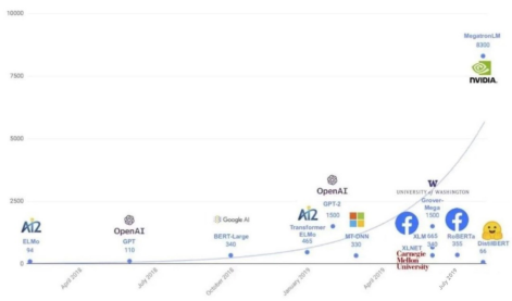
A single device is obviously not capable of training such a large model on so much training data. Let's take GPT-3 model training as an example. With eight V100 GPUs, training takes around 36 years. However, if we increase the number of V100 GPUs to 512, the training time would be reduced to almost seven months. Alternatively, by utilizing 1024 A100 GPUs, the training duration can be further reduced to just one month. Longer the time leads to higher the cost, which could be unaffordable for individuals. Given this scenario, a distributed parallel method is required to boost computing power and accelerate data processing and model training.

Solution

As mentioned above, distributed parallel strategies include data parallelism, model parallelism, and hybrid parallelism. Data parallelism splits training data into batches to train an identical model across different devices. At the end of each round of training, gradients are aggregated to update parameters. Data parallelism can be carried out either synchronously or asynchronously (through a parameter server) based on the communication mode. Hybrid parallelism is a combination of data parallelism and model parallelism.

Data Parallelism

Assume eight GPUs or Ascend NPUs are used to train an image classification model and the training data is split into 160 batches. The number of batches (min-batch) allocated to each device is 20, and each device completes training based on the allocated sample data. The obtained gradients vary with different data samples on devices. Therefore, the gradients need to be aggregated (summing and averaging) to ensure that the result is the same as that of single-device training. Then, the parameters are updated.

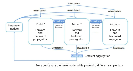
Data parallelism depends on collective communication. The preceding example uses the Broadcast and AllReduce communication primitives. Broadcast distributes data to different devices, while AllReduce aggregates gradients from different devices.

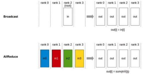
In addition to the Broadcast and AllReduce operators, AllGather, ReduceScatter, and AlltoAll can facilitate parallel processing of multiple types of data: AllGather concatenates the input tensors of each device in dimension 0 to unify the output values. ReduceScatter sums up the inputs of each device, splits the data based on the number of devices in dimension 0, and distributes the data to the corresponding device. AlltoAll divides inputs into blocks in a specific dimension, sends the blocks to other ranks in sequence, receives inputs from other ranks, and concatenates data in a specific dimension in sequence.

The preceding operators process data in synchronous mode, where model parameters are updated after gradient aggregation of different devices and then a new round of training is started. Conversely, the asynchronous mode updates model weights and parameters asynchronously, that is, workers on a single device does not need to wait for other workers, and the next round of training can be started after gradient aggregation and parameter update. A typical application of the asynchronous mode is the parameter server architecture. Specifically, a parameter server manages model weights, continuously updates the model based on worker training gradients, and pushes a new model to workers to start a next round of training.

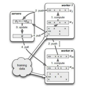
Compared with the synchronous mode, the asynchronous mode has a higher throughput without waiting for slow workers. However, the training may not cover all data once a worker fails. As a result, it is unknown that how many epochs are processed. To address this issue, the checkpoint mode is proposed to periodically save data or enable resumable training. A parameter server may also be implemented synchronously.

Model Parallelism

Data parallelism cannot deal with models with hundreds and thousands of billions of parameters, such as GPT-3, which cannot be carried by a single device. Therefore, inter-layer (models are divided onto multiple hardware devices by layer) or intra-layer (model parameters at each layer are divided onto multiple hardware devices) parallelism is required.

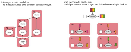
As shown on the left, network models vary with different devices in the inter-layer parallel mode. For example, the embedding layer is executed on P0, and P1, P2, and P3 are used to calculate the subsequent fully connected layers. On the contrary, intra-layer parallelism does not change the network structure. Instead, the model parameters of each layer are divided onto different devices for parallel processing. As shown on the right, the matrix calculation of each layer is divided onto devices P0 to P3. 04 Cases Most AI frameworks supports distributed parallelism. For example, the MindSpore framework supports data parallelism, model parallelism, and hybrid parallelism. For model parallelism, the framework supports automatic, semi-automatic, and manual modes according to actual situations. On MindSpore, different parallel strategies can be set using the context module:

from mindspore.communication import init, get_rank, get_group_size from mindspore import context init() device_num = get_group_size() rank = get_rank() print("rank_id is {}, device_num is {}".format(rank, device_num)) context.reset_auto_parallel_context() # Configure one of the following modes: # Data parallelism context.set_auto_parallel_context(parallel_mode=context.ParallelMode.DATA_PARALLEL) # Semi-automatic parallelism # context.set_auto_parallel_context(parallel_mode=context.ParallelMode.SEMI_AUTO_PARALLEL) # Automatic parallelism # context.set_auto_parallel_context(parallel_mode=context.ParallelMode.AUTO_PARALLEL) # Manual parallelism # context.set_auto_parallel_context(parallel_mode=context.ParallelMode.HYBRID_PARALLEL)

Once configured, the distributed parallel modes can be used for different scenarios. Data Parallelism

The following is an example of data parallelism on a simple network. If developers need to modify the network during data parallelism, they only need to set ParallelMode.DATA_PARALLEL to data parallelism through context.

import numpy as np from mindspore import Tensor, context, Model, Parameter from mindspore.communication import init from mindspore import ops, nn class DataParallelNet(nn.Cell): def __init__(self): super(DataParallelNet, self).__init__() # Initialize weights. weight_init = np.random.rand(512, 128).astype(np.float32) self.weight = Parameter(Tensor(weight_init)) self.fc = ops.MatMul() self.reduce = ops.ReduceSum() def construct(self, x): x = self.fc(x, self.weight) x = self.reduce(x, -1) return x init() # Set the parallel mode to data parallelism. context.set_auto_parallel_context(parallel_mode=context.ParallelMode.DATA_PARALLEL) net = DataParallelNet() model = Model(net) model.train(*args, **kwargs)

On MindSpore, automatic acceleration is enabled for data parallelism, which monitors whether training bottlenecks occur on the data side. If so, the degree of parallelism of data processing operators and operator queue length (affecting memory usage) are automatically adjusted based on the state of resources (memory and CPU), accelerating data processing. To enable auto tuning, the dataset module needs to be imported by inputting the following code:

import mindspore.dataset as ds ds.config.set_enable_autotune(True)

The following displays the ResNet-50 performance after auto tuning is enabled. As shown in the command output, the time for training an epoch is reduced from 72s to 17s:

[WARNING] [auto_tune.cc:297 Analyse] Op (MapOp(ID:3)) is slow, input connector utilization=0.975806, output connector utilization=0.298387, diff= 0.677419 > 0.35 threshold. [WARNING] [auto_tune.cc:253 RequestNumWorkerChange] Added request to change "num_parallel_workers" of Operator: MapOp(ID:3)From old value: [2] to new value: [4]. [WARNING] [auto_tune.cc:309 Analyse] Op (BatchOp(ID:2)) getting low average worker cpu utilization 1.64516% < 35% threshold. [WARNING] [auto_tune.cc:263 RequestConnectorCapacityChange] Added request to change "prefetch_size" of Operator: BatchOp(ID:2)From old value: [1] to new value: [5]. epoch: 1 step: 1875, loss is 1.1544309 epoch time: 72110.166 ms, per step time: 38.459 ms epoch: 2 step: 1875, loss is 0.64530635 epoch time: 24519.360 ms, per step time: 13.077 ms epoch: 3 step: 1875, loss is 0.9806979 epoch time: 17116.234 ms, per step time: 9.129 ms

Another typical use of data parallelism is parameter servers. Based on its own communication primitives, MindSpore implements synchronous parameter servers. A parameter server generally consists of three components: Server, Worker, and Scheduler. Their functions are as follows:

Server: saves model weights and backward propagation gradients, and uses an optimizer to update a model based on the gradients uploaded by Worker. Worker: performs forward and backward propagation of the network. Backward propagation gradients are uploaded to Server through the Push API, and the model updated by Server is downloaded to Worker through the Pull API. Scheduler: establishes the communication relationship between Server and Worker. The following describes how to use MindSpore to complete LeNet distributed training on Ascend 910 through a parameter server: 1. Prepare the training script: Use the LeNet training code in the MindSpore model code repository and the MNIST dataset. https://gitee.com/mindspore/models/tree/r1.6/official/cv/lenet

2. Set parameters for the parameter server training mode: Use the following code to start the parameter server mode, initialize the network, and update the training weights through the parameter server.

context.set_ps_context(enable_ps=True) network = LeNet5(cfg.num_classes) network.set_param_ps()

3. Configure the scripts for starting the three components.

Scheduler script (scheduler.sh):

#!/bin/bash export MS_SERVER_NUM=1 export MS_WORKER_NUM=1 export MS_SCHED_HOST=XXX.XXX.XXX.XXX export MS_SCHED_PORT=XXXX export MS_ROLE=MS_PSERVER python train.py --device_target=Ascend --data_path=path/to/dataset

Server script (server.sh):

Worker script (worker.sh):

#!/bin/bash export MS_SERVER_NUM=1 export MS_WORKER_NUM=1 export MS_SCHED_HOST=XXX.XXX.XXX.XXX export MS_SCHED_PORT=XXXX export MS_ROLE=MS_WORKER python train.py --device_target=Ascend --data_path=path/to/dataset

4. Start training and view the results. Run the sh Scheduler.sh > scheduler.log 2>&1 &, sh Server.sh > server.log 2>&1 &, and sh Worker.sh > worker.log 2>&1 & commands to start the three components. Then, view the communication logs of Server and Worker in the scheduler.log file.

The server node id:b5d8a47c-46d7-49a5-aecf-d29d7f8b6124,node ip: xxx.xxx.xxx..xxx,node port:46737 assign rank id:0 The worker node id:55e86d4b-d717-4930-b414-ebd80082f541 assign rank id:1 Start the scheduler node is successful!

If the training results are displayed in worker.log, the LeNet training is successful in the parameter server mode.

epoch: 1 step: 1, loss is 2.302287 epoch: 1 step: 2, loss is 2.304071 epoch: 1 step: 3, loss is 2.308778 epoch: 1 step: 4, loss is 2.301943 ...

Summary

With the explosion of model parameters and training data, distributed parallelism is becoming the optimal choice for developers to accelerate model training. Distributed training can be further optimized in terms of hardware and practice. For example, you can use dedicated hardware, NPUs (such as Ascend), and TPUs (Google). Different distributed parallel modes affect training speed. In addition, the batch size of the training data needs to be properly selected. If a min-batch contains a large amount of data, the number of training iterations can be reduced, compromising the convergence speed of gradient descent and overall progress. During actual model training, select proper hardware, a parallel mode, and hyperparameters to accelerate the process.

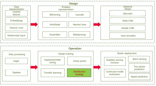
The feature hash mode, though applicable to some scenarios, causes model precision loss. The mode is not suitable when data is clearly classified, the vocabulary is relatively small (around 1000), and cold start does not exist. Modulo is a lossy operation. In the feature hash mode, different categories are placed in the same bucket, affecting data accuracy. The inference error becomes large when the classified data is particularly unbalanced. For example, the traffic of Xi'an Xianyang International Airport is two orders of magnitude larger than that of Yulin Yuyang Airport Airport. If they are placed in the same bucket and are processed as one type of code, the model will bias the Xi'an Xianyang International Airport, resulting in deviations in the prediction of wait time.

There are two ways to mitigate the precision loss:

1. Add aggregation features: If the distribution of categorical variables is skewed or a small number of buckets causes many conflicts, you can add aggregation features as the input of the model. For example, for each airport, the probability of a punctual flight can be found in the training dataset and added to the model as a feature, to avoid losing airport information when hashing airport code. In some cases, you can abandon the feature of airport names, as the relative frequency of flight punctuality may be sufficient.

2. Adjust the number of buckets as a hyperparameter to achieve precision balance.

References

[1]https://www.zhihu.com/question/498275802/answer/2221187242

[2]https://www.jiqizhixin.com/articles/2020-04-24-5

[3]https://www.oreilly.com/library/view/machine-learning-design/9781098115777/

[4]https://mindspore.cn/docs/programming\_guide/zh-CN/r1.6/distributed\_training\_ops.html

[5]https://gitee.com/mindspore/docs/tree/r1.6/docs/sample\_code/distributed\_training