MindSpore Case Study | Adversarial Attacks with Fast Gradient Sign Method

With continuous development and evolution of data, computing power, and theories in recent years, deep learning has been widely applied in many fields involving images, texts, voice, and autonomous driving. Meanwhile, people are getting more and more concerned about the security issues of various models in use, because AI models are vulnerable to intentional or unintentional attacks and generate incorrect results. In this case, we will use the fast gradient sign method (FGSM) attack as an example to demonstrate how to attack and mislead a model.

01 Preparation

Visit the MindSpore official siteto install MindSpore.

Obtain the installation commands.

In the Notebook, add the following commands before the first code cell and execute them:

pip install --upgrade pip
conda install mindspore-gpu=1.9.0 cudatoolkit=10.1 -c mindspore -c conda-forge
pip install mindvision

02 Adversarial Example Definition

Szegedy first proposed the concept of adversarial examples in 2013. Small perturbations that cannot be perceived by humans are added to original examples, deteriorating the performance of deep models. Such examples are adversarial examples. For example, after a noise is added to the image that should be predicted as panda, the model predicts the image as gibbon:

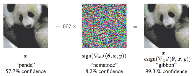
The image comes from Explaining and Harnessing Adversarial Examples.

03 Attack Methods

Attacks on models can be classified from the following aspects:

1. Information that can be obtained by attackers:

l White-box attack: Attackers have all knowledge and access permissions on a model, including the model structure, weight, input, and output. Attackers can interact with the model system in the process of generating adversarial attack data. Due to that attackers completely master information about models, they can design specific attack algorithms based on the features of the attacked model.

l Black-box attack: Contrary to white-box attacks, attacks only obtain limited information about models. Attackers know nothing about the structure or weight of the model and know only part of the input and output.

2. Attackers' purposes:

l Targeted attack: Attackers misguide the model result into a specific category.

l Untargeted attack: Attackers only want to generate incorrect results and do not care about new results.

The FGSM attack used in this case is a white-box attack method that can be either a targeted or untargeted attack.

For more model security functions, see MindSpore Armour. Currently, MindSpore Armour supports multiple adversarial example generation methods, such as FGSM, LLC, and Substitute Attack, and provides adversarial example robustness, fuzz testing, and privacy protection and evaluation modules to enhance model security.

FGSM Attack

During the training of a classification network, a loss function is defined to measure the distance between the model output value and the actual label of the example. The model gradient is computed through backward propagation. The network parameters are updated through gradient descent to reduce the loss value and improve the model accuracy.

FGSM is a simple and efficient method for generating adversarial examples. Different from the training process of a normal classification network, FGSM computes the gradient ∇xJ(θ,x,y) of the loss to the input. The gradient indicates the sensitivity of the loss to the input change.

Then, the preceding gradient is added to the original input to increase the loss value. As a result, the classification effect of the reconstructed input examples deteriorates, and the attack is successful. Another requirement of adversarial examples is that the difference between the generated example and the original example must be as small as possible. The sign function can be used to make the image modification as even as possible.

The generated adversarial perturbation may be expressed by using the following formula:

η=εsign(∇xJ(θ)) (1)

Adversarial examples can be formulated as follows:

x′=x+εsign(∇xJ(θ,x,y)) (2)

· x: original input image that is correctly classified as "Pandas"

· y: output of x

· θ: model parameter

· ε: attack coefficient

· J(θ,x,y): loss of the training network

· ∇xJ(θ): backward propagation gradient

04 Data Processing

In this case, MNIST is used to train LeNet with the qualified accuracy, and then the FGSM attack mentioned above is executed to deceive the network model and enable the model to implement incorrect classification.

Use the following sample code to download and decompress a dataset to a specified location.

from mindvision.dataset import Mnist

# Download and process the MNIST dataset.
download_train = Mnist(path="./mnist", split="train", shuffle=True, download=True)
download_eval = Mnist(path="./mnist", split="test", download=True)

dataset_train = download_train.run()
dataset_eval = download_eval.run()

The directory structure of the downloaded dataset files is as follows:

./mnist
├── test
│   ├── t10k-images-idx3-ubyte
│   └── t10k-labels-idx1-ubyte
└── train
    ├── train-images-idx3-ubyte
    └── train-labels-idx1-ubyte

05 Training LeNet

In the experiment, LeNet is used to complete image classification as a demo model. You need to define the network and use the MNIST dataset for training.

Define LeNet:

from mindvision.classification.models import lenet

network = lenet(num_classes=10, pretrained=False)

Define an optimizer and a loss function:

import mindspore.nn as nn

net_loss = nn.SoftmaxCrossEntropyWithLogits(sparse=True, reduction='mean')
net_opt = nn.Momentum(network.trainable_params(), learning_rate=0.01, momentum=0.9)

Define network parameters:

import mindspore as ms

config_ck = ms.CheckpointConfig(save_checkpoint_steps=1875, keep_checkpoint_max=10)
ckpoint = ms.ModelCheckpoint(prefix="checkpoint_lenet", config=config_ck)

Train LeNet:

from mindvision.engine.callback import LossMonitor

model = ms.Model(network, loss_fn=net_loss, optimizer=net_opt, metrics={'accuracy'})
model.train(5, dataset_train, callbacks=[ckpoint, LossMonitor(0.01, 1875)])

Test the current network. You can see that LeNet has reached a high accuracy.

acc = model.eval(dataset_eval)
print("{}".format(acc))

06 Implementing FGSM

After the accurate LeNet is obtained, the FGSM attack is used to load noise in the image and perform the test again.

Compute a backward gradient using the loss function:

class WithLossCell(nn.Cell):
    """Package the network and loss functions."""

    def __init__(self, network, loss_fn):
        super(WithLossCell, self).__init__()
        self._network = network
        self._loss_fn = loss_fn

    def construct(self, data, label):
        out = self._network(data)
        return self._loss_fn(out, label)

class GradWrapWithLoss(nn.Cell):
    """Compute a backward gradient using the loss function."""

    def __init__(self, network):
        super(GradWrapWithLoss, self).__init__()
        self._grad_all = ops.composite.GradOperation(get_all=True, sens_param=False)
        self._network = network

    def construct(self, inputs, labels):
        gout = self._grad_all(self._network)(inputs, labels)
        return gout[0]

Then, implement the FGSM attack according to formula (2):

import numpy as np

class FastGradientSignMethod:
    """Implement FGSM."""

    def __init__(self, network, eps=0.07, loss_fn=None):
        # Initialize variables.
        self._network = network
        self._eps = eps
        with_loss_cell = WithLossCell(self._network, loss_fn)
        self._grad_all = GradWrapWithLoss(with_loss_cell)
        self._grad_all.set_train()

    def _gradient(self, inputs, labels):
        # Calculate the gradient.
        out_grad = self._grad_all(inputs, labels)
        gradient = out_grad.asnumpy()
        gradient = np.sign(gradient)
        return gradient

    def generate(self, inputs, labels):
        # Implement FGSM.
        inputs_tensor = ms.Tensor(inputs)
        labels_tensor = ms.Tensor(labels)
        gradient = self._gradient(inputs_tensor, labels_tensor)
        # Generate perturbation.
        perturbation = self._eps*gradient
        # Generate the images after perturbation.
        adv_x = inputs + perturbation
        return adv_x

    def batch_generate(self, inputs, labels, batch_size=32):
        # Process the dataset.
        arr_x = inputs
        arr_y = labels
        len_x = len(inputs)
        batches = int(len_x / batch_size)
        res = []
        for i in range(batches):
            x_batch = arr_x[i*batch_size: (i + 1)*batch_size]
            y_batch = arr_y[i*batch_size: (i + 1)*batch_size]
            adv_x = self.generate(x_batch, y_batch)
            res.append(adv_x)
        adv_x = np.concatenate(res, axis=0)
        return adv_x

Reprocess the images from the test set in the MINIST dataset:

images = []
labels = []
test_images = []
test_labels = []
predict_labels = []

ds_test = dataset_eval.create_dict_iterator(output_numpy=True)

for data in ds_test:
    images = data['image'].astype(np.float32)
    labels = data['label']
    test_images.append(images)
    test_labels.append(labels)
    pred_labels = np.argmax(model.predict(ms.Tensor(images)).asnumpy(), axis=1)
    predict_labels.append(pred_labels)

test_images = np.concatenate(test_images)
predict_labels = np.concatenate(predict_labels)
true_labels = np.concatenate(test_labels)

07 Running Attack

It can be seen from the FGSM attack formula that, the larger the attack coefficient ε, the greater the change to the gradient. If the value of ε is 0, the attack effect is not reflected.

η=εsign(∇xJ(θ)) (3)

Observe the attack effect when ε is 0:

import mindspore.ops as ops

fgsm = FastGradientSignMethod(network, eps=0.0, loss_fn=net_loss)
advs = fgsm.batch_generate(test_images, true_labels, batch_size=32)

adv_predicts = model.predict(ms.Tensor(advs)).asnumpy()
adv_predicts = np.argmax(adv_predicts, axis=1)
accuracy = np.mean(np.equal(adv_predicts, true_labels))
print(accuracy)

Set ε to 0.5 and try to run the attack:

fgsm = FastGradientSignMethod(network, eps=0.5, loss_fn=net_loss)
advs = fgsm.batch_generate(test_images, true_labels, batch_size=32)

adv_predicts = model.predict(ms.Tensor(advs)).asnumpy()
adv_predicts = np.argmax(adv_predicts, axis=1)
accuracy = np.mean(np.equal(adv_predicts, true_labels))
print(accuracy)

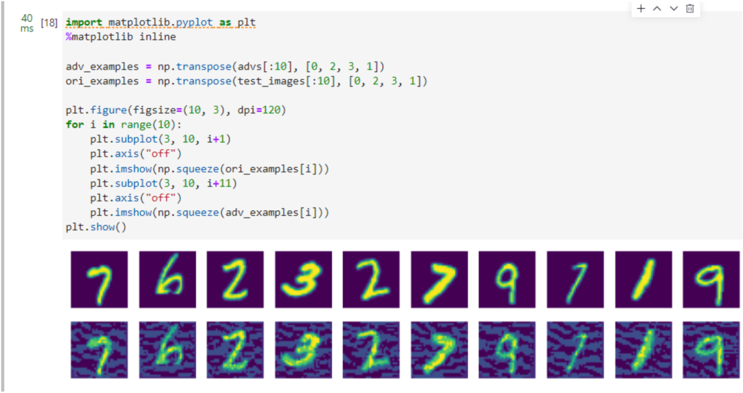
The preceding result shows that the accuracy of the LeNet model is greatly reduced.

The following shows the actual form of the attacked image. It can be seen that the image changes slightly, but the accuracy decreases greatly in the test.

import matplotlib.pyplot as plt
%matplotlib inline

adv_examples = np.transpose(advs[:10], [0, 2, 3, 1])
ori_examples = np.transpose(test_images[:10], [0, 2, 3, 1])

plt.figure(figsize=(10, 3), dpi=120)
for i in range(10):
    plt.subplot(3, 10, i+1)
    plt.axis("off")
    plt.imshow(np.squeeze(ori_examples[i]))
    plt.subplot(3, 10, i+11)
    plt.axis("off")
    plt.imshow(np.squeeze(adv_examples[i]))
plt.show()