Idea Sharing (19): Practising Electromagnetic Inversion of Ground Penetrating Radars
Idea Sharing (19): Practising Electromagnetic Inversion of Ground Penetrating Radars
2022-05-27
Ground penetrating radars (GPRs) [1] provide a geophysical method of detecting the attributes and distribution of materials with antennas to transmit and receive high-frequency electromagnetic waves. Featuring high precision, high efficiency, and no destruction, the method has been applied in many fields including archaeology, mineral exploration, disaster geological investigation, geotechnical engineering investigation, engineering quality inspection, building structure inspection, and target detection. MindSpore Elec [2] has been focused on the forward problem: Knowing the structure and attributes of the target to be simulated, it calculates physical quantities such as electromagnetic fields and scattering parameters. The electromagnetic inversion of GPRs is a classical inverse problem, which deduces the structure and attributes of the target based on the received electromagnetic wave signal. When using traditional methods like noise suppression and time variable gain, researchers need to select proper methods and parameters based on different characteristics of the method and target. Therefore, researchers must be highly qualified and the expected effect is hard to achieve. This paper mainly introduces how to use the data-driven AI method of MindSpore Elec to solve the electromagnetic inverse problem of GPRs.
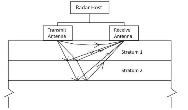
Figure 1 Principle of detection with GPRs
MindSpore Elec Electromagnetic Inversion Practice
1. Data Generation
gprMax[3] is traditional open-source electromagnetic simulation software based on Finite-Difference Time-Domain (FDTD). It can be used for modeling and solving for GPRs' forward problems. Therefore, gprMax is used to generate data for training and inference.
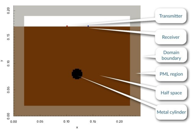
Figure 2 cylinder_Ascan_2D model
First, install the gprMax 3.1.5 open-source software. The user_models directory in the gprMax source code provides the basic application model of the GPR. Here, we use the http://cylinder_Ascan_2D.in model.
Figure 2 shows the general process of this model: The transmitter emits electromagnetic waves, and when the electromagnetic waves reach the metal cylinder, the signals are reflected back to the receiver. Users infer the position of the metal cylinder based on the received electromagnetic signals. In the http://cylinder_Ascan_2D.in file, #domain indicates the simulation area (x, y, and z, in meters), #dx_dy_dz indicates the grid size (in meters), #time_window indicates the simulation time (in seconds), #material indicates the model attribute, #waveform indicates the waveform (amplitude and frequency) of the transmit source, #hertzian_dipole indicates the position of the transmit source, #rx indicates the position of the receive source, #box indicates the background medium, #cylinder indicates the position and material attribute of the metal cylinder, and #geometry_view exports the geometric information of the model to a file. For details, see [4] and [5].
http://cylinder\_Ascan\_2D.in file:
#title: A-scan from a metal cylinder buried in a dielectric half-space
#domain: 0.240 0.210 0.002
#dx_dy_dz: 0.002 0.002 0.002
#time_window: 3e-9
#material: 6 0 1 0 half_space
#waveform: ricker 1 1.5e9 my_ricker
#hertzian_dipole: z 0.100 0.170 0 my_ricker
#rx: 0.140 0.170 0
#box: 0 0 0 0.240 0.170 0.002 half_space
#cylinder: 0.120 0.080 0 0.120 0.080 0.002 0.010 pec
#geometry_view: 0 0 0 0.240 0.210 0.002 0.002 0.002 0.002 cylinder_half_space n
Second, by moving the position of the metal cylinder (other conditions remain unchanged), we generated more than 300 sample data records.
2. Modeling and Training
It is concluded from the results of the forward problem that, the Ez, Hx, and Hy electromagnetic field components play a role in the two-dimensional electromagnetic issue. Therefore, we construct a neural network mapping from Ez, Hx, Hy to the position of the metal cylinder, that is, cylinder_pos ([x, y]) = Net ([Ez, Hx, Hy]).
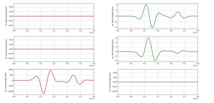
Figure 3 Forward results of electromagnetic exploration
The neural network model is described as follows:
class Model(nn.Cell):

    def __init__(self):

        super(Model,self).__init__()

        self.conv1 = nn.Conv1d(3,10,3)

        self.relu = nn.ReLU()

        self.maxpool = nn.MaxPool1d(2,2)

        self.conv2 = nn.Conv1d(10,32,3)

        self.tanh = nn.Tanh()

        self.conv3 = nn.Conv1d(32,64,3)

        self.fc1 = nn.Dense(5056,1200)

        self.fc2 = nn.Dense(1200,100)

        self.fc3 = nn.Dense(100,2)

        self.reshape = ops.Reshape()

    def construct(self,x):

        x1 = self.relu(self.conv1(x))

        x2 = self.maxpool(x1)

        x3 = self.tanh(self.conv2(x2))

        x3 = self.maxpool(x3)

        x4 = self.relu(self.conv3(x3))

        x4 = self.maxpool(x4)

        x5 = self.reshape(x4, (x.shape[0],-1))

        x6 = self.relu(self.fc1(x5))

        x7 = self.fc2(x6)

        output = self.fc3(x7)

        return output
3. Result
Figure 4 shows the training result, where X_pos and Y_pos are respectively the horizontal and vertical coordinates of the metal cylinder. The training loss can reach 2.6 x 10⁻⁶, and the relative error reaches 8.7 x 10⁻³.
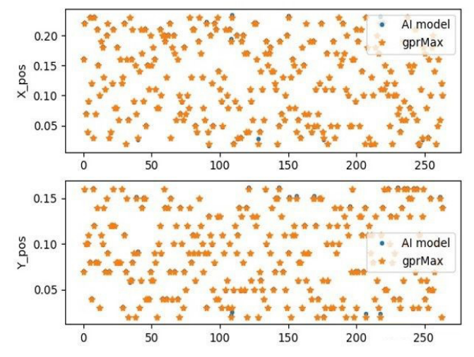
Figure 4 AI training result
Figure 5 shows the inference result. The inference loss reaches 10–4, and the relative error reaches 5 x 10⁻².
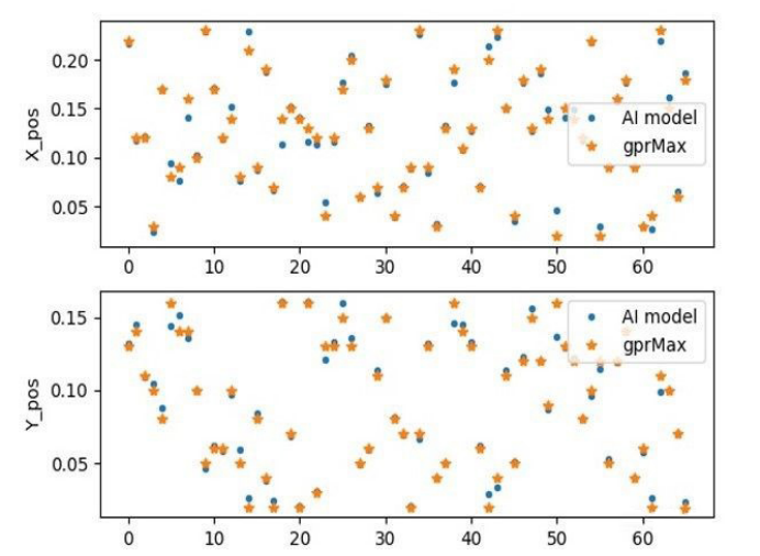
Figure 5 AI inference result
Summary and Prospects
We have made a preliminary exploration of the electromagnetic inverse problem and found that AI methods can effectively solve such problems. Later, we will open the codes above in the MindSpore Elc repository and further study more complex scenarios. Anyone interested in AI electromagnetic simulation is welcome to join us to explore this topic.
References:
1. Study on Spectrum Characteristics of Ground Penetrating Radars in Water-Rich Crushed Zone in Karst Area
3. https://github.com/gprMax/gprMax
4. Introductory (2D) models