MindSpore Made Easy Deep Learning Series - Classical Convolutional Neural Networks

June 10, 2022

This blog describes two more complicated classical convolutional neural networks (CNNs), LeNet and AlexNet.

Classic CNN - LeNet

LeNet-5, a handwritten font recognition model, was first proposed in 1994 and was one of the earliest CNNs. LeNet-5 uses such operations as convolution, parameter sharing, and pooling to extract features, reducing large computing costs. It then uses a fully-connected neural network (FCNN) for recognition and classification.

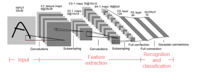
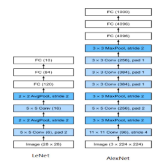
LeNet-5 network structure

LeNet-5 consists of seven layers (excluding the input layer). Ci represents the convolutional layers, Si represents the sub-sampling (pooling) layers, and Fi represents the fully-connected layers. The size of each original input image is 32 x 32 pixels.

1. Layer C1 (convolutional layer)

This layer uses six convolution kernels. The size of each convolution kernel is 5 x 5. Six feature maps can be obtained.

(1) Feature map size

Every convolution kernel (5 x 5) is convolved with every input image (32 x 32 pixels), so that the size of each obtained feature map is (32 – 5 + 1) x (32 – 5 + 1) = 28 x 28 pixels.

Knowledge point: The convolution kernels and input images are matched and calculated region by region based on the convolution kernel size. After the matching, the size of each input image decreases because the convolution kernel cannot cross the boundary at the image edge and only one match is allowed. After the calculation, the image size changes to Cr x Cc = (Ir – Kr + 1) x (Ic – Kc + 1), where Cr, Cc, Ir, Ic, Kr, and Kc respectively represent row and column sizes of the result image after convolution, the input image, and the convolution kernel.

(2) Number of parameters

Because parameters (weights) are shared, all neurons of a convolution kernel use the same parameters. The total number of parameters is (5 x 5 + 1) x 6 = 156, where 5 x 5 is the convolution kernel size and 1 is the offset.

(3) Number of connections

The size of a convolutional image is 28 x 28 pixels. That is, a feature map has 28 x 28 neurons. The parameter quantity of each convolution kernel is (5 x 5 + 1) x 6, and the number of connections at this layer is (5 x 5 + 1) x 6 x 28 x 28 = 122304.

2. Layer S2 (downsampling or pooling layer)

(1) Feature map size

This layer mainly performs pooling or feature mapping (that is, feature dimension reduction) and the pooling unit is 2 x 2. After pooling, the size of the six feature maps changes to 14 x 14.

Because pooling units do not overlap, after aggregation statistics of 2 x 2 pooling in the pooling area, a new feature value is recalculated for every two rows and two columns, which is equivalent to halving the feature map size. That is, a convolved 28 x 28 feature map becomes a 14 x 14 image.

The calculation process at this layer is as follows:

a) Add the values in the 2 x 2 unit.

b) Multiply the added values by the training parameter w.

c) Add the bias parameter b (feature maps share the same w and b).

d) Use the Sigmoid value (S function: 0-1) as the corresponding unit value.

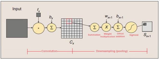
Convolution and pooling

(2) Number of parameters

At layer S2, because all feature maps share the same w and b parameters, 2 x 6 = 12 parameters are required.

(3) Number of connections

The image size after downsampling is 14 x 14 pixels. That is, each feature map at layer S2 has 14 x 14 neurons. The number of connections of each pooling unit is 2 x 2 + 1 (1 is the offset), and the total number of connections at this layer is (2 x 2 + 1) x 14 x 14 x 6 = 5880.

3. Layer C3 (convolutional layer)

This layer has 16 convolution kernels, and the size of each kernel is 5 x 5.

(1) Feature map size

Similar to the analysis at layer C1, the size of each feature map at layer C3 is calculated as (14 – 5 + 1) x (14 – 5 + 1) = 10 x 10.

(2) Number of parameters

Note that C3 and S2 are only partially connected. In this way, more features can be extracted. The following figure shows the connection rule.

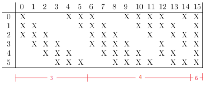
For example, the first column indicates that feature map 0 at layer C3 is connected only to feature maps 0, 1, and 2 at layer S2. The calculation process is as follows:

a) Use three convolution templates to convolve with three feature maps at layer S2, respectively.

b) Sum up the convolution results.

c) Add an offset.

d) Use Sigmoid to obtain the convolved feature maps.

Other columns are similar (some have three convolution templates, some have four, and some have six). Therefore, the quantity of parameters at this layer is (5 x 5 x 3 + 1) x 6 + (5 x 5 x 4 + 1) x 9 + 5 x 5 x 6 + 1 = 1516.

(3) Number of connections

The size of each feature map after convolution is 10 x 10 pixels, and the number of parameters is 1516. Therefore, the number of connections is 1516 x 10 x 10 = 151600.

4. Layer S4 (downsampling or pooling layer)

(1) Feature map size

Similar to the analysis at layer S2, the size of each pooling unit is 2 x 2. This layer has 16 feature maps, and the size of each feature map is 5 x 5 pixels.

(2) Number of parameters

Similar to the calculation at layer S2, the number of required parameters is 16 x 2 = 32.

(3) Number of connections

(2 x 2 + 1) x 5 x 5 x 16 = 2000

5. Layer C5 (convolutional layer)

(1) Feature map size

This layer has 120 convolution kernels, and the size of each convolution kernel is also 5 x 5. Therefore, there are 120 feature maps.

Because at layer S4, the size of each feature map is 5 x 5 pixels and the size of each convolution kernel is 5 x 5, the feature map size at layer C5 can be calculated as (5 – 5 + 1) x (5 – 5 + 1) = 1 x 1. That is, layer C5 becomes fully connected. However, this is only a coincidence because this layer may not be fully connected if the original input image is large in size.

(2) Number of parameters

The number of parameters at this layer is 120 x (5 x 5 x 16 + 1) = 48120.

(3) Number of connections

The size of each feature map at this layer is 1 x 1. Therefore, the number of connections is 48120 x 1 x 1 = 48120.

6. Layer F6 (fully-connected layer)

(1) Feature map size

Layer F6 has 84 units because the output layer corresponds to a 7 x 12 bitmap, as shown in the following figure. -1 indicates the white color, and 1 indicates the black color. The black and white of each symbol in the bitmap form a code.

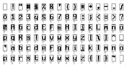
This layer has 84 feature maps. The size of each feature map is 1 x 1 pixels, which is the same as that at layer C5. Therefore, this layer is also fully connected.

(2) Number of parameters

Because this layer is fully connected, the number of parameters is calculated as (120 + 1) x 84 = 10164. Like any classical neural network, layer F6 calculates the dot product between the input and weight vectors, adds an offset, and transfers to the Sigmoid function to obtain the result.

(3) Number of connections

Because this layer is fully connected, the number of connections is the same as that of parameters, that is, 10164.

7. Output layer

The output layer is also a fully-connected layer that contains 10 nodes, representing digits 0 to 9. If the value of the ith node is 0, the result of network-enabled recognition is the digit i.

(1) Feature map size

This layer adopts the radial basis function (RBF) network connection mode. Assuming that x is the input to the previous layer and y is the output of the RBF, the RBF function is calculated as follows:

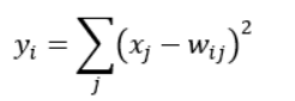
The value of Wij in the preceding formula is determined by the bitmap code of i, where i ranges from 0 to 9, and j ranges from 0 to 7 x 12 – 1. The closer the RBF output value is to 0, the closer the recognition result is to the digit i.

(2) Number of parameters

Because this layer is fully connected, the number of parameters is calculated as 84 x 10 = 840.

(3) Number of connections

Because this layer is fully connected, the number of connections is the same as that of parameters, that is, 840.

LeNet convolutional layers are used to identify spatial patterns in images, such as lines and object parts. Pooling layers are used to reduce the sensitivity of convolutional layers to locations. After convolutional and maximum pooling layers are alternately used, fully-connected layers are connected to perform image classification. This shows that a CNN trained by gradient descent could achieve the most advanced results of handwritten digit recognition at that time.

Classic CNN - AlexNet

The first typical CNN is LeNet-5, but the first network that attracts public attention is AlexNet.

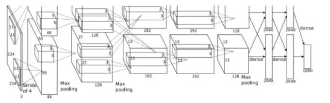
AlexNet network structure

The network has eight layers, including five convolutional layers and three fully-connected layers.

1. Layer 1: convolutional layer C1. The inputs are 224 x 224 x 3 images. The number of convolution kernels is 96. The size of each convolution kernel is 11 x 11 x 3. The stride is 4. The pad is 0, indicating that the edge is not padded.

The size of each convolved image is as follows:

Width = (224 + 2 x pad – kernel_size)/stride + 1 = 54

Height = (224 + 2 x pad – kernel_size)/stride + 1 = 54

Dimension = 96

After local response normalization (LRN) and pooling (pool_size = (3, 3), stride = 2, pad = 0) on the input images, you can finally obtain the feature maps of the first-layer convolution.

2. Layer 2: convolutional layer C2. The inputs are the feature maps obtained after convolution at layer C1. The number of convolution kernels is 256. The size of each convolution kernel is 5 x 5 x 48. The pad is 2, and the stride is 1. After LRN and max. pooling (pool_size = (3, 3), stride = 2) on the input feature maps, you can obtain the outputs.

3. Layer 3: convolutional layer C3. The inputs are the outputs of layer C2. The number of convolution kernels is 384. The size of each convolution kernel is 3 x 3 x 256. The pad is 1. No LRN or pooling is performed at layer C3.

4. Layer 4: convolutional layer C4. The inputs are the outputs of layer C3. The number of convolution kernels is 384. The size of each convolution kernel is 3 x 3. The pad is 1. No LRN or pooling is performed at layer C4.

5. Layer 5: convolutional layer C5. The inputs are the outputs of layer C4. The number of convolution kernels is 256. The size of each convolution kernel is 3 x 3 x 3. The pad is 1. Max. pooling (pool_size = (3, 3), stride = 2) is directly performed.

6. Layers 6, 7, and 8 are fully-connected layers, which use ReLU and Dropout. The number of neurons at each layer is 4096, and the final output Softmax is 1000.

AlexNet developed LeNet's ideas and applied CNNs' basic principles to deep and wide networks.

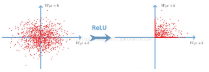
In AlexNet, ReLU is used as the activation function, and it has been verified that ReLU outperforms Sigmoid in deep networks because it can solve the gradient vanishing problem.

ReLU function: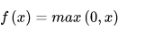

In addition, AlexNet uses overridden pooling operations. Common pooling layers do not overlap, so pool_size and stride values are generally the same. For example, for an 8 x 8 image, if the pooling layer size is 2 x 2, the result image obtained after pooling is 4 x 4. This is a non-overridden pooling operation. If stride is smaller than pool_size, an overridden pooling operation is generated, which is similar to a convolutional operation. During model training, an overridden pooling layer is less likely to be overfitting.

Overfitting is one of the serious problems faced by neural networks. AlexNet adopts the data expansion and Dropout methods to deal with this problem. At any layer, some neurons are randomly deleted based on a defined probability, but the quantity of neurons at the input and output layers remains unchanged. Then, parameters are updated according to the neural network learning method. In the next iteration, some neurons are randomly deleted again until training ends.

Summary

The design concepts of AlexNet and LeNet are similar, but there are significant differences. First, AlexNet is much deeper than the relatively small LeNet-5. AlexNet consists of eight layers, including five convolutional layers, two fully-connected hidden layers, and one fully-connected output layer. Second, AlexNet uses ReLU instead of Sigmoid as its activation function.

Higher layers of AlexNet are built on the underlying representation to represent larger features such as eyes, noses, grass leaves, and so on. Higher layers can also detect entire objects, such as a person, an airplane, a dog, or a Frisbee. The final hidden neurons can learn the comprehensive representation of each image, so that data belonging to different classes can be easily distinguished.

AlexNet proves for the first time that the learned features can surpass the features of manual design. AlexNet is much better than LeNet in terms of results, especially in the convenience of processing large-scale data. The advent of AlexNet also started the large-scale application of deep learning in the field of computer vision. Generally, we can consider it as the boundary between shallow neural networks and deep neural networks.

There are many other classic CNNs, such as VGG, GoogLeNet, and ResNet. Let's learn and use.