Machine Learning with MindSpore Large-Scale Machine Learning

1. The Necessity of Large-Scale Datasets

If you have a low-bias model, increasing the size of the dataset can help achieve better results. How do we handle a training set of 1 million examples?

Take a linear regression model as an example. To perform a single step of gradient descent, you need to calculate the sum of the squared error of the training set. Generally, the computational expense would be very large for 20 iterations.

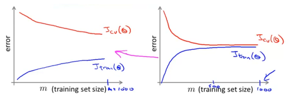
Before putting the effort into training a model on 1 million examples, we should check whether such a large training set is necessary, and if training on 1,000 examples might do just as well. In this case, plotting the learning curves will help a lot.

2. Stochastic Gradient Descent

If you have confirmed that a large-scale training set is necessary, you can try using stochastic gradient descent instead of batch gradient descent.

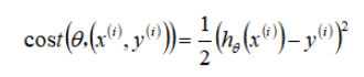
In stochastic gradient descent, the cost function is defined as the cost of a parameter with respect to a single training example.

The first step of stochastic gradient descent is to randomly shuffle the training set. Then, the following procedure is performed:

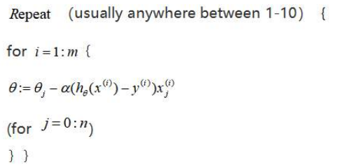
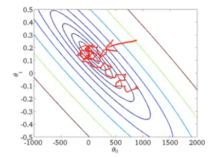
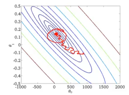
Instead of performing summation over all training examples, stochastic gradient descent scans through the training examples one by one and slightly modify the parameter θ accordingly. Multiple passes are performed before an iteration of stochastic gradient descent is completed. Of course, every coin has two sides. Not every iteration takes the parameters in the "right" direction. Although stochastic gradient descent generally moves the parameters in the direction of the global minima, the algorithm does not actually converge but wanders around continuously in a region close to the global minima.

3. Mini-batch Gradient Descent

Mini-batch gradient descent is an algorithm in between batch gradient descent and stochastic gradient descent. In mini-batch gradient descent, b examples (the mini-batch size) are used in each iteration to update the parameter θ.

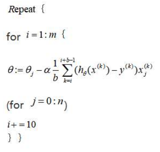
A typical choice for the value of b is a number between 2 and 100. By using appropriate vectorization to compute the derivative terms over the b examples, you can sometimes use the numerical linear algebra libraries to parallelize your gradient computations, and the overall performance of the algorithm is not affected (same as that of stochastic gradient descent).

4. Stochastic Gradient Descent Convergence

How do we tune the learning rate α for stochastic gradient descent?

To check if batch gradient descent converges, we plot the cost function J as a function of the number of iterations of gradient descent to see whether J is decreasing. However, for a large-scale the training set, this approach is not feasible because of the huge computational cost.

In stochastic gradient descent, the cost of a training example is computed before θ is updated. For every x iterations, we can plot the costs averaged over the processed x examples.

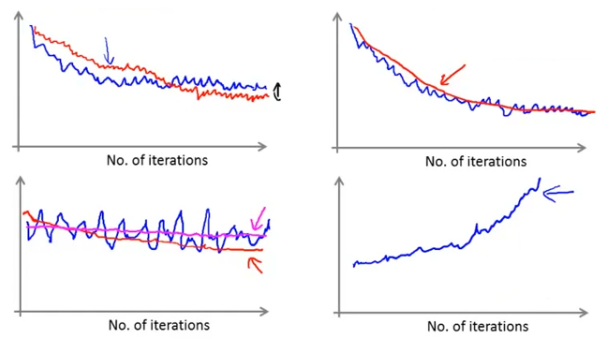
When plotting the function, we may get a graph that is noisy and not decreasing (the blue curve in the lower left figure). By increasing α, the graph will be smoother and possibly show a trend of decreasing (the red curve in the lower left figure). If the graph is still noisy and not decreasing (the pink curve in the lower left figure), the problem could be with the model itself.

If you get a graph that is increasing (the lower right figure), you need to use a smaller learning rate α.

You can also slowly decrease the learning rate αover iterations, for example:

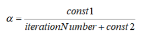
As the algorithm gets closer to the global minima, the learning rate decreases, allowing the algorithm to converge to the global minima instead of meandering around it. However, this approach requires you to tune extra parameters (const1 and const2) and is unnecessary in most cases.

To summarize, we talked about a method for approximately monitoring the performance of stochastic gradient descent during cost function optimization. This method does not periodically scan the entire training set to compute the cost function. Instead, it focuses on the last x examples. You can use this method to ensure that stochastic gradient descent works properly and converges or to tune the learning rate α.

5. Online Learning

Online learning is a new large-scale machine learning mechanism. The online learning mechanism allows us to model problems.

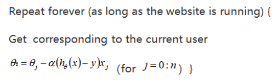
Many large websites use different versions of online learning algorithms to learn from the flood of users accessing the websites. If you have a continuous stream of data generated by a continuous stream of users, you can use an online learning algorithm to learn user preferences to optimize the decisions on your website.

Online learning algorithms refer to the learning of data streams rather than offline static datasets. Many websites have continuous user streams. For each user, the website wants to learn algorithms smoothly without storing data.

Assume a website providing shipping services. Users specify the origin and destination on the website to obtain the prices for shipping their packages. A user may choose (y=1, a positive example) or refuse (y=0, a negative example) to use a shipping service based on the price offered by the website. A learning algorithm can be used to help the website to price shipping services reasonably.

To build a model to predict the probability that a user chooses to use the shipping service, the price needs to be captured as one of the features. Other features include the distance, origin and destination, and specific user data. The model output is p(y=1).

After the algorithm learns from an example, the example is discarded and not stored. An advantage of this method is that the algorithm can adapt to changing user preferences by updating the model continuously according to the user behavior.

Moreover, every time the user interacts with the website, multiple datasets are generated. For example, if the user chooses two of the three provided shipping options, three training examples are generated. Then, the online learning algorithm uses these examples to update the parameters.

Any of these problems can be formulated as a standard machine learning problem, where the website runs for a few days and saves the data as a fixed training set to run a learning algorithm on it. But the cost for storing data increases as data volume grows. There is really no need to save a fixed training set. Instead, you can use an online learning algorithm to learn continuously from data generated by users. Online learning is similar to stochastic gradient descent except that instead of scanning through a fixed training set, online learning obtains one example from the users, learns from it, and discards it and moves on. Another advantage of online learning is that if the pool of users is changing, or the website tries to predict a changing target, online learning can slowly adapt the learned hypothesis to the latest user behavior.

6. MapReduce

MapReduce is very important to large-scale machine learning. Using batch gradient descent to find the optimal solution of a large-scale dataset involves computing sums of partial derivatives and costs over the entire training set, which is computationally expensive. The MapReduce approach splits the dataset onto multiple computers, each of which processes a sub-set, and combines the results together.

Specifically, if a learning algorithm can be expressed as computing the sums of functions over the training set, the computing task can be distributed to multiple computers (or multiple CPU cores of a computer) to speed up training.

For example, for a training set of 400 examples, the task of computing the sums of functions of batch gradient descent can be distributed to four computers as follows:

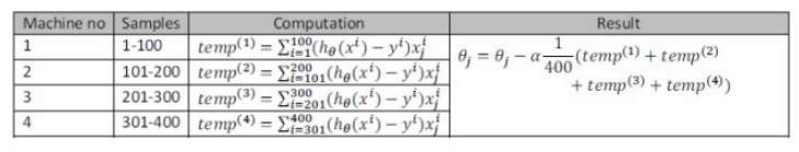
Many advanced linear algebra function libraries can use multiple cores of a CPU to process matrix operations in parallel, which is also the reason why the appropriate vectorization of the algorithm is so important.