Writing BERT in Hundreds of Lines of Code Using MindSpore, Impressive!
Writing BERT in Hundreds of Lines of Code Using MindSpore, Impressive!
October 12, 2021
Author: Lv Yufeng | Source: Zhihu
If you ask me how I think of MindSpore 1.5, I'd say it is impressive considering its capability of writing BERT in just hundreds of lines of code. As a milestone NLP model launched in 2018, BERT has always been a must-try for machine learning enthusiasts, deconstructed and analyzed for countless times. In this blog I'll try to explain why BERT is so important and how MindSpore simplifies its training process. If you haven't tried MindSpore before and are somewhat interested, please read through.
1 Do I Really Need 1000 Lines of Code for BERT Implementation?
I used MindSpore quite a lot, especially for the implementation of pre-trained NLP models. For reference, I checked ModelZoo, a library of popular networks with implementation code. I was shocked that for BERT, nearly a thousand lines of code are required. That was quite a complex process, almost the opposite from MindSpore claims to be, easy-to-use and efficient. I can't stop but wonder, is there an easier way?
First let's look at the official implementation code (gitee.com/mindspore/models/blob/master/official/nlp/bert/src/bert_model.py). Even if we take out the code comments, the implementation is still complex and lengthy. Later, when I need to migrate the checkpoints from HuggingFace to MindSpore, I wrote a much shorter version myself. The official implementation example can surely be compressed, to hundreds of lines of code, as a matter of fact.
2 The BERT Model
BERT, short for Bidirectional Encoder Representation from Transformers, is also the name of the cute yellow Muppet character on Sesame Street. You got to admit, Google's geeks got some talent in giving names, right?

Bert from the Sesame Street
As the name suggests, BERT is a bidirectional Transformer encoder, which absorbs the advantages of GPT and ELMo, and makes full use of the feature extraction capability of Transformer. Back in 2018 and 2019, BERT really ranked top on those famous dataset benchmarks, and got so much attention. It is yet the one legendary SOTA model you wouldn't want to miss. Next, I'll use my version of code to build a lightweight BERT and explain from the most basic components of formulas, graphics, and code. I'll not introduce the basic knowledge of Transformer or pre-trained language models in detail here. Let's start now.
3 Multi-head Attention
Since this is just a blog, I will not analyze the differences between BERT and Transformer in embedding as in formal papers. Nor will I detail the pre-training tasks. Instead, I will start from the basic module implementation.
The basic framework of the BERT model consists of the encoders of the transformer. Therefore, I will briefly describe the self-attention and multi-head attention modules in the transformer. The first is self-attention, also called scaled dot-product attention in some papers. The formula is as follows:
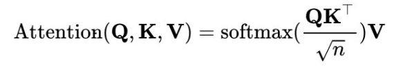
The self-attention is calculated by Q (query matrix), K (key matrix), and V (value matrix) inputs, which are obtained by performing linear transformation on the same input through the fully connected layer. The code is as follows:
class ScaledDotProductAttention(Cell):

    def __init__(self, d_k, dropout):

        super().__init__()

        self.scale = Tensor(d_k, mindspore.float32)

        self.matmul = nn.MatMul()

        self.transpose = P.Transpose()

        self.softmax = nn.Softmax(axis=-1)

        self.sqrt = P.Sqrt()

        self.masked_fill = MaskedFill(-1e9)

        if dropout > 0.0:

            self.dropout = nn.Dropout(1-dropout)

        else:

            self.dropout = None


    def construct(self, Q, K, V, attn_mask):

        K = self.transpose(K, (0, 1, 3, 2))

        scores = self.matmul(Q, K) / self.sqrt(self.scale) # scores : [batch_size x n_heads x len_q(=len_k) x len_k(=len_q)]

        scores = self.masked_fill(scores, attn_mask) # Fills elements of self tensor with value where mask is one.

        attn = self.softmax(scores)

        context = self.matmul(attn, V)

        if self.dropout is not None:

            context = self.dropout(context)

        return context, attn
After Q*K^T is scaled, a masked_fill operation is performed, which is implemented with reference to the PyTorch version. In the initial input sequence, replace the calculated result with a number near 0 at the position of Padding 0 in the input sequence, for example, -1e-9 in the preceding code. In addition, the dropout operation is performed to increase the robustness of the model.
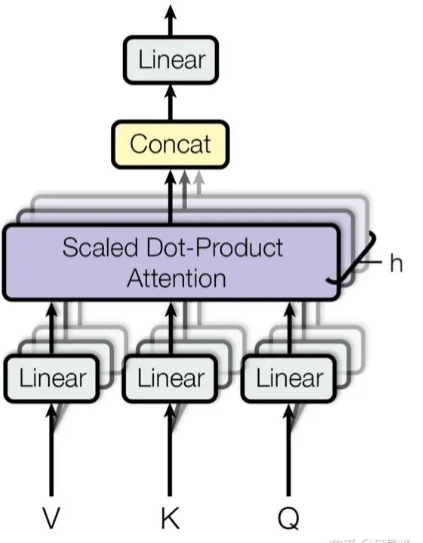
Multi-head Attention
After completing the scaled dot-product attention, let's look at the implementation of the multi-headed attention mechanism. In fact, the original single Q, K, and V are projected into h Q's, K's, and V's. Therefore, the generalization capability of the model is enhanced without changing the calculation amount. The term may be interpreted as an ensemble of a plurality of heads in an ensemble model, or alternatively, as a convolution operation with multiple channels. To some extent, CNN was the inspiration for multi-head attention. The implementation code is as follows:
class MultiHeadAttention(Cell):

    def __init__(self, d_model, n_heads, dropout):

        super().__init__()

        self.n_heads = n_heads

        self.W_Q = Dense(d_model, d_model)

        self.W_K = Dense(d_model, d_model)

        self.W_V = Dense(d_model, d_model)

        self.linear = Dense(d_model, d_model)

        self.head_dim = d_model // n_heads

        assert self.head_dim * n_heads == d_model, "embed_dim must be divisible by num_heads"

        self.layer_norm = nn.LayerNorm((d_model, ), epsilon=1e-12)

        self.attention = ScaledDotProductAttention(self.head_dim, dropout)

        # ops

        self.transpose = P.Transpose()

        self.expanddims = P.ExpandDims()

        self.tile = P.Tile()


    def construct(self, Q, K, V, attn_mask):

        # q: [batch_size x len_q x d_model], k: [batch_size x len_k x d_model], v: [batch_size x len_k x d_model]

        residual, batch_size = Q, Q.shape[0]

        q_s = self.W_Q(Q).view((batch_size, -1, self.n_heads, self.head_dim))

        k_s = self.W_K(K).view((batch_size, -1, self.n_heads, self.head_dim))

        v_s = self.W_V(V).view((batch_size, -1, self.n_heads, self.head_dim))

        # (B, S, D) -proj-> (B, S, D) -split-> (B, S, H, W) -trans-> (B, H, S, W)

        q_s = self.transpose(q_s, (0, 2, 1, 3)) # q_s: [batch_size x n_heads x len_q x d_k]

        k_s = self.transpose(k_s, (0, 2, 1, 3)) # k_s: [batch_size x n_heads x len_k x d_k]

        v_s = self.transpose(v_s, (0, 2, 1, 3)) # v_s: [batch_size x n_heads x len_k x d_v]


        attn_mask = self.expanddims(attn_mask, 1)

        attn_mask = self.tile(attn_mask, (1, self.n_heads, 1, 1)) # attn_mask : [batch_size x n_heads x len_q x len_k]


        # context: [batch_size x n_heads x len_q x d_v], attn: [batch_size x n_heads x len_q(=len_k) x len_k(=len_q)]

        context, attn = self.attention(q_s, k_s, v_s, attn_mask)

        context = self.transpose(context, (0, 2, 1, 3)).view((batch_size, -1, self.n_heads * self.head_dim)) # context: [batch_size x len_q x n_heads * d_v]

        output = self.linear(context)

        return self.layer_norm(output + residual), attn # output: [batch_size x len_q x d_model]
Q, K, and V first pass through the dense layer for linear transformation, then pass through reshape (view) to switch to multi-heads, and then transpose to meet the requirement of being sent to ScaledDotProductAttention. Concatenate the obtained output. Note that the concatenation operation is not explicitly performed. Instead, it restores shape[-1] of the context to heads*hidden_size through the view. In addition, the Add&Norm operation is added to the return operation, that is, the corresponding residual and Norm calculation in the encoder structure. For details, see the next section.
4 Transformer Encoder
After the basic multi-head attention is done, we can complete the rest to construct a single-layer encoder. Allow me to briefly describe the structure of the single-layer encoder here. The transformer encoder consists of the poswise feed forward layer and multi-head attention layer, and the residual operation is performed on the input and output of each layer (y = f(x) + x), ensuring that the number of layers of the deep neural network does not decrease. Layer norm is also performed to mitigate gradient vanishing and explosion, thus to meet the training requirements of the deep neural network. If you wonder why I use the layer norm instead of the batch norm, feel free to google it. It's an interesting trick for Transformer construction.
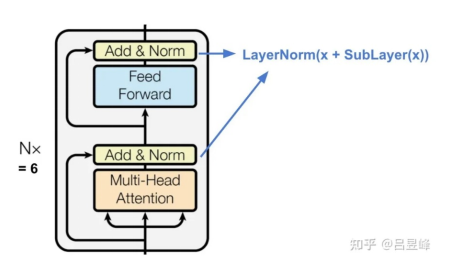
Transformer Encoder
After talking about the encoder structure, we need to implement the missing poswise feed forward layer. Similar to the multi-head attention layer, you need to integrate residual and layer norm. The implementation code is as follows:
class PoswiseFeedForwardNet(Cell):

    def __init__(self, d_model, d_ff, activation:str='gelu'):

        super().__init__()

        self.fc1 = Dense(d_model, d_ff)

        self.fc2 = Dense(d_ff, d_model)

        self.activation = activation_map.get(activation, nn.GELU())

        self.layer_norm = nn.LayerNorm((d_model,), epsilon=1e-12)


    def construct(self, inputs):

        residual = inputs

        outputs = self.fc1(inputs)

        outputs = self.activation(outputs)


        outputs = self.fc2(outputs)

        return self.layer_norm(outputs + residual)
Concatenate the multi-head attention layer to the poswise feed forward layer to obtain the encoder:
class BertEncoderLayer(Cell):

    def __init__(self, d_model, n_heads, d_ff, activation, dropout):

        super().__init__()

        self.enc_self_attn = MultiHeadAttention(d_model, n_heads, dropout)

        self.pos_ffn = PoswiseFeedForwardNet(d_model, d_ff, activation)


    def construct(self, enc_inputs, enc_self_attn_mask):

        enc_outputs, attn = self.enc_self_attn(enc_inputs, enc_inputs, enc_inputs, enc_self_attn_mask)

        enc_outputs = self.pos_ffn(enc_outputs)

        return enc_outputs, attn
Based on the configured parameters such as the number of layers, hidden_size, and head, concatenate the encoders at n layers to complete the BERT encoder. The nn.CellList container is used for implementation.
class BertEncoder(Cell):

    def __init__(self, config):

        super().__init__()

        self.layers = nn.CellList([BertEncoderLayer(config.hidden_size, config.num_attention_heads, config.intermediate_size, config.hidden_act, config.hidden_dropout_prob) for _ in range(config.num_hidden_layers)])


    def construct(self, inputs, enc_self_attn_mask):

        outputs = inputs

        for layer in self.layers:

            outputs, enc_self_attn = layer(outputs, enc_self_attn_mask)

        return outputs
5 Constructing BERT
After the encoders are complete, we can assemble a complete BERT model. The preceding sections describe the implementation of the Transformer encoder structure. The BERT model differs primarily from the Transformer model in its backbone. The first difference is the processing of embedding.
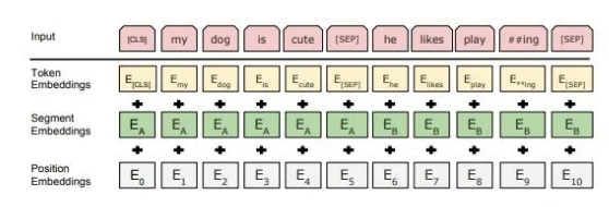
This figure shows how the text input is sent to the BERT embedding to obtain the hidden layer representation, which is obtained by adding three different embeddings:
Token Embedding: It is the most common word vector. The first placeholder is [CLS], which is used to express the encoding of the entire input text after subsequent encoding. It is used in classification tasks, therefore becomes CLS, that is, classifier. In addition, the [SEP] placeholder is used to separate two different sentences of the same input, and [PAD] indicates padding.
Segment Embedding: It is used to distinguish two different sentences of the same input, and added to perform the next sentence predict task.
Position Embedding: Similar to the Transformer, position embedding cannot be used to retain the location information naturally, which needs to be manually encoded. Transformers use trigonometric functions, but here, the index corresponding to the location is sent directly to the embedding layer. (There is no essential difference between the two. Position embedding can be simpler and more direct.)
Now, we can directly use nn.Embedding to process the embeddings. The corresponding code is as follows:
class BertEmbeddings(Cell):

    def __init__(self, config):

        super().__init__()

        self.tok_embed = Embedding(config.vocab_size, config.hidden_size)

        self.pos_embed = Embedding(config.max_position_embeddings, config.hidden_size)

        self.seg_embed = Embedding(config.type_vocab_size, config.hidden_size)

        self.norm = nn.LayerNorm((config.hidden_size,), epsilon=1e-12)


    def construct(self, x, seg):

        seq_len = x.shape[1]

        pos = mnp.arange(seq_len) # mindspore.numpy

        pos = P.BroadcastTo(x.shape)(P.ExpandDims()(pos, 0))

        seg_embedding = self.seg_embed(seg)

        tok_embedding = self.tok_embed(x)

        embedding = tok_embedding + self.pos_embed(pos) + seg_embedding

        return self.norm(embedding)
Here, mindspore.numpy.arange is used to generate the location index. Other operations are simple invocation and matrix addition.
After the embedding layer is complete, concatenate the encoder and the output pooler to form a complete BERT model. The code is as follows:
class BertModel(Cell):

    def __init__(self, config):

        super().__init__(config)

        self.embeddings = BertEmbeddings(config)

        self.encoder = BertEncoder(config)

        self.pooler = Dense(config.hidden_size, config.hidden_size, activation='tanh')


    def construct(self, input_ids, segment_ids):

        outputs = self.embeddings(input_ids, segment_ids)

        enc_self_attn_mask = get_attn_pad_mask(input_ids, input_ids)

        outputs = self.encoder(outputs, enc_self_attn_mask)

        h_pooled = self.pooler(outputs[:, 0])

        return outputs, h_pooled
Here, a dense layer is used to perform the pooler operation on the output whose position is 0, that is, the input text representation corresponding to the [CLS] placeholder, for subsequent classification tasks.
6 BERT for Pre-training Tasks
The essence of the BERT model lies in task design rather than model architecture. BERT designs two pre-training tasks for "unsupervised" NLP model training.
6.1 Next Sentence Predict
First, let's analyze the NSP task. I added the NSP task to enhance the model for downstream tasks with two input sentences, such as QA or NLI. As the name implies, the pre-training task concatenates sentences A and B as the input. Half of B is correct and will be used as the next sentence of A, and the other half randomly selects text that is not the next sentence. The prediction task uses the binary classification, predicting whether B is the next sentence of A. The sample code is as follows:
class BertNextSentencePredict(Cell):

    def __init__(self, config):

        super().__init__()

        self.classifier = Dense(config.hidden_size, 2)


    def construct(self, h_pooled):

        logits_clsf = self.classifier(h_pooled)

        return logits_clsf
6.2 Masked Language Model
Token of the mask. This task is different from the traditional language model (or GPT) in that it is bidirectional.
This function is used as the target function. The masked token is predicted based on the context, which naturally complies with the form of blank filling.
Data preprocessing is not involved herein, and therefore mask and replacement ratio are not described in detail. The corresponding implementation is simple, which is actually Dense+activation+LayerNorm+Dense. The implementation code is as follows:
class BertMaskedLanguageModel(Cell):

    def __init__(self, config, tok_embed_table):

        super().__init__()

        self.transform = Dense(config.hidden_size, config.hidden_size)

        self.activation = activation_map.get(config.hidden_act, nn.GELU())

        self.norm = nn.LayerNorm((config.hidden_size, ), epsilon=1e-12)

        self.decoder = Dense(tok_embed_table.shape[1], tok_embed_table.shape[0], weight_init=tok_embed_table)


    def construct(self, hidden_states):

        hidden_states = self.transform(hidden_states)

        hidden_states = self.activation(hidden_states)

        hidden_states = self.norm(hidden_states)

        hidden_states = self.decoder(hidden_states)

        return hidden_states
Combine the two tasks to complete the pre-trained BERT model.
class BertForPretraining(Cell):

    def __init__(self, config):

        super().__init__(config)

        self.bert = BertModel(config)

        self.nsp = BertNextSentencePredict(config)

        self.mlm = BertMaskedLanguageModel(config, self.bert.embeddings.tok_embed.embedding_table)


    def construct(self, input_ids, segment_ids):

        outputs, h_pooled = self.bert(input_ids, segment_ids)

        nsp_logits = self.nsp(h_pooled)

        mlm_logits = self.mlm(outputs)

        return mlm_logits, nsp_logits
The above code is an example of how I build a BERT model by using MindSpore. You can see that each module completely corresponds to the formula or diagram, the implementation of a single module is about 10 to 20 lines, and the overall implementation code is between 150 and 200 lines. Compared with the official example in ModelZoo, my version is much shorter, which is actually a proof that MindSpore can be quite efficient and concise.
7 Code Comparison
Due to the space limit, I selected one code screenshot for comparison.
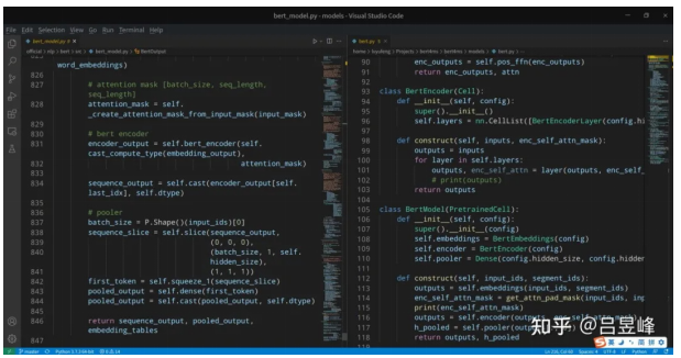
The left part is the official implementation code, while the right part is my version. The same BERT model can be simply implemented using just hundreds of lines of code. After multiple iterations, MindSpore has been evolved to a mature deep learning framework, with comprehensive operator support and enhanced front-end expression usability. In the past, only PyTorch can implement BERT in a few hundred lines of code. Now, with MindSpore 1.5, we can do the same.
As a MindSpore user and a community contributor, I understand that the official implementation samples are based on earlier versions of MindSpore. But for newcomers or developers who just want to give MindSpore a shot, they might lose interest seeing the code implementation in ModelZoo. In fact, MindSpore 1.2 and later versions can compete with PyTorch in model construction efficiency. I hope this blog can inspire more people to try MindSpore. If you have better code implementation, feel free to submit PRs at https://github.com/mindspore-ai/mindspore or https://gitee.com/mindspore/mindspore.
8 Summary
First, from my personal experience, MindSpore did continuously improving its development experience and usability. From MindSpore 0.7 to MindSpore 1.5, I spent lesser time in building the same model. However, as a growing open source project, there can be defects and a huge room for improvement. I wrote this blog to tell you, if only you try MindSpore by yourself, you can see its great potential. Besides, finding bugs and optimize them is always a thing for geeks.
LLMs are not the mount Everest. The Transformer architecture is WYSIWYG. Try them yourself, and you'll see the beauty of NLP.