AI Engineering 04- Why Is the AI Industry in Need of Parallel Distributed Training?

June 29, 2022

Massive computing power is required for training AI models. With the growing volume of data and increasing scale of parameters, standalone devices fail to provide the computing power required for efficient model training. Therefore, parallel distributed training is proposed.

This article discusses why parallel distributed training is needed, its strategies, and the implementation mechanism and advantages of MindSpore approaches.

Why Parallel Distributed Training

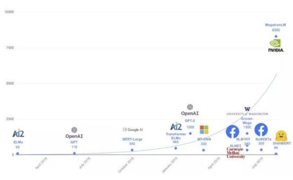
After the release of OpenAI GPT-3, major vendors launched their foundation models, marking a new round of fierce technology competition in the AI field. Building a foundation model is not easy. It involves complex algorithms and requires massive amount of data and computing power. Take the GPT series as an example:

1. GPT-1 contains hundreds of millions of parameters, trained on the BookCorpus dataset that contains 10,000 books of 2.5 billion words.

2. GPT-2 contains 1.5 billion parameters, trained on the WebText dataset that consists of data of 8 million web pages linked from Reddit. The total amount of data is about 40 GB after cleansing.

3. GPT-3 is the first model that contains over 10 billion parameters. The corpus is based on the Common Crawl dataset (400 billion tokens), WebText2 (19 billion tokens), BookCorpus (67 billion tokens), and Wikipedia (3 billion tokens).

A single device is obviously not capable of training such a large model on so much data. For example, it takes approximately 36 years to train GPT-3 using eight V100 GPUs, 7 months using 512 V100 GPUs, or 1 month using 1024 A100 GPUs. Longer training time costs higher, which makes the training of a large model unaffordable for common developers. Therefore, parallel distributed training is proposed to enhance computing power, accelerate data processing, and speed up model training.

Parallel Distributed Training Strategies

Mainstream parallel distributed training strategies in the industry include data parallelism (where data is split up), model parallelism (where the model is split up), and hybrid parallelism.

○ Data parallelism: Data is split into batches and allocated to each compute unit for training.

○ Model parallelism: The model is sharded. This strategy consists of operator-level parallelism, pipeline parallelism, and optimizer parallelism.

○ Operator-level parallelism: The input tensors of an operator are distributed to multiple devices for distributed computing. This strategy distributes data samples and model parameters to multiple devices so that large models training becomes feasible and the overall training speed improves as benefited from computing resources across the entire cluster. Using operator-level parallelism, a developer can set a shard strategy for each operator in the forward network. The framework performs shard modeling on each operator and its input tensors based on the operator shard strategy to keep the operator computing logic mathematically unchanged after sharding.

○ Pipeline parallelism: In operator-level parallelism, a communication domain is established across the entire cluster, where each device communicates with all the other devices. When there are a lot of devices in the cluster, such a practice could reduce the communication efficiency and overall performance. This problem can be addressed by pipeline parallelism, which divides a neural network into multiple stages that are executed by different sets of devices. In this way, a device communicates only within a communication domain that covers a limited number of devices. Pipeline parallelism enables the devices to efficiently communicate with each other and process layered network structures. However, the resource utilization of pipeline parallelism is relatively low because devices can be idle from time to time.

○ Optimizer parallelism: During training in data parallelism or operator-level parallelism mode, copies of the same set of parameters may exist on multiple devices. As a result, optimizers on the devices perform redundant calculation when updating weights of the parameters. In this case, optimizer parallelism can distribute necessary computing workload to multiple devices to reduce the static memory overhead and computing workload of each optimizer, but the communication cost will increase.

○ Hybrid parallelism: The combination of data parallelism and model parallelism.

Implementations in MindSpore

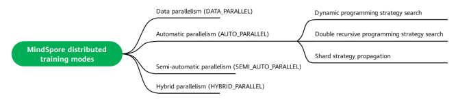
The MindSpore framework supports data parallelism, automatic parallelism (including data parallelism and operator-level parallelism), semi-automatic parallelism (manually configured operator shard strategies), and hybrid parallelism (manually sharded models).

○ Data parallelism: Use this mode if the workload of your network parameter calculation is within the allowed range of a single device. In this mode, the same network parameters are copied to each device, and different training data is input to the devices.

○ Automatic parallelism: Use this mode if the workload of your network parameter calculation cannot be covered by a single device and you do not know how to configure the operator shard strategy. In this mode, MindSpore automatically configures the shard strategy for each operator. In terms of strategy search algorithms, MindSpore supports the following:

○ Dynamic programming strategy search: This algorithm finds the optimal strategy demonstrated by its cost model but requires a long time to search for the parallelism strategy for a large network. The cost model is created by modeling the training time based on the memory-based computation and communication overheads of Ascend 910 processors.

○ Double recursive programming strategy search: The optimal strategy can be generated instantly even for a large network or for a large-scale multi-device sharding scenario. Its symbolic cost model can flexibly adapt to different accelerator clusters.

○ Shard strategy propagation: Strategies are propagated from operators with configured shard strategy to those without. During propagation, the algorithm selects the strategy that causes the least tensor redistribution communication.

○ Semi-automatic parallelism: Use this mode if the calculation workload of your neural network parameters cannot be covered by a single device, and there is a high requirement for performance after sharding. You can specify the shard strategy for each operator to achieve better training performance.

○ Hybrid and parallelism: Use this mode if you know about how to design the logic and implementation of parallel training. You can define communication operators including AllGather in the network.

In practice, you can use the context.set_auto_parallel_context() interface to set the mode of distributed training.

# Data parallelism

context.set_auto_parallel_context(parallel_mode=context.ParallelMode.DATA_PARALLEL)

# Semi-automatic parallelism

context.set_auto_parallel_context(parallel_mode=context.ParallelMode.SEMI_AUTO_PARALLEL)

# Automatic parallelism

context.set_auto_parallel_context(parallel_mode=context.ParallelMode.AUTO_PARALLEL)

# Hybrid parallelism

context.set_auto_parallel_context(parallel_mode=context.ParallelMode.HYBRID_PARALLEL)

1. Data Parallelism

Assume eight GPUs or Ascend NPUs are used to train an image classification model and the training dataset is split into 160 batches. 20 batches (mini-batches) are allocated to each device for training. Each device obtains distinct gradients because of different sample data. The gradients need to be aggregated (through summing and averaging) in order to achieve the same result as that of single-device training. The parameters are then updated based on the aggregated result. The process is as follows:

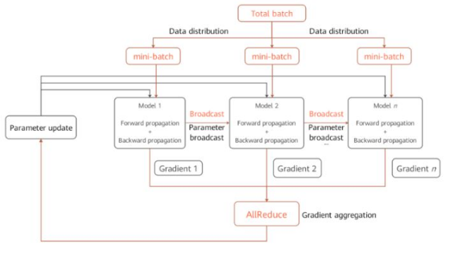
○ Establishing communication: A communication group is established across devices through a communication library (for example, HCCL of Ascend or NCCL of NVIDIA). The mindspore.communication.init interface can be used for communication initialization.

○ Distributing data: The core of data parallelism is to split datasets by samples and distribute them to different devices. All dataset loading interfaces provided by the mindspore.dataset module have the num_shards and shard_id parameters. Based on these parameters, the MindSpore framework splits a dataset into multiple sub-sets, performs cyclic sampling, and collects data of the batch size to each device. When data is insufficient, the sampling restarts from the beginning.

○ Structuring network: Like single-device training, each device independently trains the model of the same network structure during forward and backward propagation.

○ Aggregating gradients: To ensure calculation logic consistency, the AllReduce operator is inserted after gradient calculation to aggregate gradients across devices.

○ Updating parameters: After gradient aggregation, model parameters on each device are updated based on the same gradient before a new round of training.

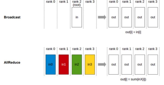
Data parallelism depends on collective communication. In the preceding example, the Broadcast and AllReduce communication primitives are used. Broadcast distributes data to the devices, and AllReduce aggregates gradients of the devices:

2**.** Model Parallelism

Model parallelism can be implemented automatically or semi-automatically. Types of model parallelism include inter-layer parallelism (a model is sharded into layers and allocated to multiple devices) and intra-layer parallelism (model parameters of each layer are distributed to multiple devices). The following figure shows the differences between the two types. In inter-layer parallelism, each device executes a different network layer. In intra-layer parallelism, the network structure is not changed. Instead, the model parameters of each layer are distributed to different devices.

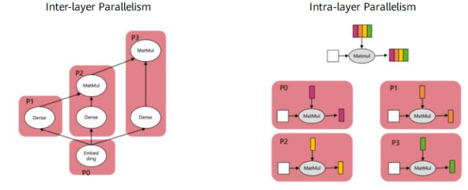
As you can see from the figure, model parallelism is more difficult to implement than data parallelism. In data parallelism, only the data is split up, and the network structure is not changed. In model parallelism, the model is sharded into layers, or parameters of each layer are distributed. When splitting a model manually, a developer needs to consider:

○ How to ensure that the sharded model can fit into the memory of a single device?

○ How to balance the model sharding granularity and efficiency, because devices communicate with each other more frequently in model parallelism.

○ How to ensure that tensors after model sharding are in the form of slices? How to choose the dimension for sharding to ensure the mathematical consistency between models before and after sharding?

MindSpore provides automatic, semi-automatic, and hybrid parallel training to help implement parallelism algorithms using single-device scripts, reducing the difficulty of distributed training and improving training performance. The following figure shows the principle and process of parallel distributed training in MindSpore:

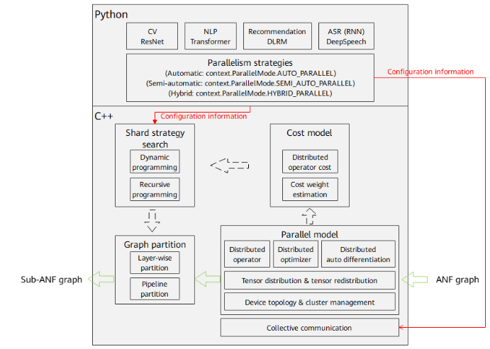
1. Parallelism strategy configuration: The front-end API is used to set automatic parallel training strategies. Different parallelism strategies (automatic, semi-automatic, and hybrid) determine different shard strategies and parallel model configurations. You can use the context.set_auto_parallel_context API to select a parallelism strategy.

2. Distributed operator and tensor distribution: The process of automatic parallelism traverses the input A-normal form (ANF) computational graph, and perform shard modeling on tensors based on the distributed operators to represent how the input and output tensors of an operator are distributed to each device in the cluster (tensor distribution). The shard model fully expresses the mapping between tensors and devices. You do not need to understand how the model slices are distributed on the devices. The framework automatically schedules and allocates the slices.

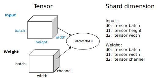
1. Tensor distribution: To obtain the tensor distribution model, each operator is configured with a shard strategy, which indicates the sharding of each input of the operator in the corresponding dimension. Generally, tensors can be sharded in any dimension as long as the value is a multiple of 2, and the even distribution principle is met. The following figure shows an example BatchMatMul operation (three-dimensional matrix multiplication). Its shard strategy consists of two tuples, indicating how the inputs and weights are sharded, respectively. Elements in the tuples correspond to tensor dimensions one by one. 2^N indicates the number of shards, and 1 indicates that the tuple is not sharded. When data parallelism is used, that is, only the batch dimension of the input is sharded, the shard strategy can be expressed as strategy=((2^N, 1, 1),(1, 1, 1)). When model parallelism is used, that is, a non-batch dimension of the weight is split (the channel dimension in this example), the shard strategy can be expressed as strategy=((1, 1, 1),(1, 1, 2^N)). When hybrid parallelism is used, the shard strategy can be strategy=((2^N, 1, 1),(1, 1, 2^N)). Based on the shard strategy, the method of deducing the distribution model of the input and output tensors of the operator is defined in the distributed operators. The distribution model consists of device_matrix, tensor_shape, and tensor map, indicating the device matrix shape, tensor shape, and mapping between devices and tensor dimensions, respectively. The distributed operators further determine whether to insert additional computing and communication operations into the graph based on the tensor distribution model to ensure that the operator calculation logic is correct. In semi-automatic parallelism mode, you need to manually configure the shard strategy for operators. This is the biggest difference between automatic and semi-automatic parallelism modes.

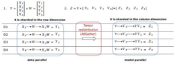
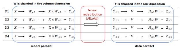
2. Tensor redistribution: When the output tensor model of the previous operator is inconsistent with the input tensor model of the next operator, calculation and communication operations are required to transform the tensor distribution. The tensor redistribution algorithm is introduced to the automatic parallelism process to deduce the transformation between tensors of any distribution. The following example uses the formula Z=(X×W)×V, that is, multiplication of two two-dimensional matrices, to demonstrate how conversion between different parallelism modes is performed.

In Figure 1, the output of the first matrix multiplication (data parallelism) is sharded in the row dimension, and the input of the second matrix multiplication (model parallelism) requires full tensors. The framework automatically inserts the AllGather operator to implement redistribution.

In Figure 2, the output of the first matrix multiplication (model parallelism) is sharded in the column dimension, and the input of the second matrix multiplication (data parallelism) is sharded in the row dimension. The framework automatically inserts a communication operator equivalent to the AlltoAll operation in collective communication to implement redistribution.

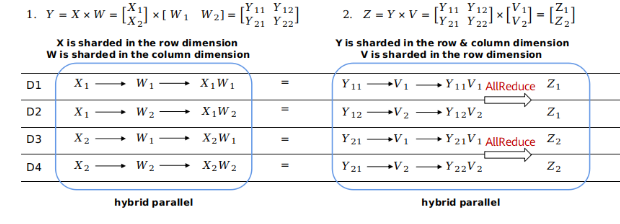
In Figure 3, the output of the first matrix multiplication is sharded in the same way as the second matrix multiplication (both are hybrid parallelism). No redistribution is required. However, in the second matrix multiplication, the related dimensions of the two inputs are sharded. Therefore, the AllReduce operator needs to be inserted to ensure the correctness.

Distributed operators and tensor distribution/redistribution are the basis of automatic parallelism. In general, this distribution representation bridges the gap between data parallelism and model parallelism. From the perspective of scripts, you only need to construct a single-device network to express the parallelism algorithm. The framework automatically shards the entire graph.

3. Shard strategy search: The automatic parallelism mode supports sharding propagation to reduce the workload of manual operator sharding. The strategies are propagated from operators with configured shard strategy to those without. Automatic shard strategy search is also supported to further reduce the workload of manual operator sharding. Automatic shard strategy search builds cost models based on the hardware platform, and calculates the computation cost, memory cost, and communication cost of a certain amount of data and specific operators based on different shard strategies. Using the dynamic programming algorithm or recursive programming algorithm and taking the memory capacity of a single device as a constraint condition, a shard strategy with optimal performance is efficiently searched out. Strategy search replaces manual model sharding and provides a high-performance sharding solution within a short period of time, greatly reducing the difficulty for parallel training.

3. Distributed automatic differentiation: The process of graph sharding includes forward and reverse network sharding. Traditionally, to manually shard a model, you need to consider backward parallel computing in addition to forward network communication. MindSpore encapsulates communication operations into operators and automatically generates backward propagation of communication operators based on the original automatic differentiation operations of the framework. Therefore, even during distributed training, you only need to pay attention to the forward propagation of the network. In this way, the actual automatic parallel training is implemented.

Automatic parallelism is user-friendly because it reduces the difficulty of parallel distributed training. The next article will be introducing how to train the ResNet-50 model using automatic parallelism based on MindSpore.