NeRF MindSpore-based NeRF Implementation

June 29, 2022

Introduction to NeRF

1. Background

The past few decades haven't witnessed major breakthroughs in the conventional computer graphics technology. However, as deep learning technologies keep advancing, the emerging neural rendering technology brings new opportunities to computer graphics, which has attracted wide attention from the academia and industry. Neural rendering is a general term for various methods for synthesizing images using deep networks. Its objective is to implement all or some modeling and rendering functions of graphics rendering. Three-dimensional (3D) reconstruction of scenes based on the neural radiation field (NeRF) is a popular direction for neural rendering recently, which aims to use neural networks to generate two-dimensional (2D) images in new angles of view. At AI summits such as CVPR and NeuIPS in 2020 and 2021, we saw dozens and hundreds of related high-level papers.

2. Network Structure

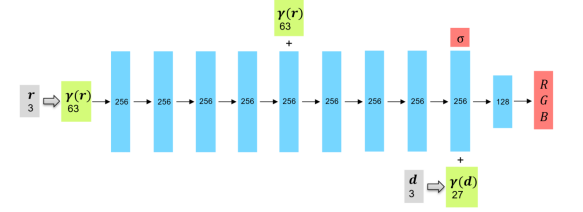
NeRF uses the multilayer perceptron (MLP) to reconstruct 3D scenes, that is, to fit functions of color distribution and optical density distribution of spatial points. In the network structure of NeRF, inputs are spatial coordinates and views of sampling points, and outputs are corresponding densities and RGB values.

Because changes of the color \boldsymbol{c}c and the optical density \sigmaσ are drastic in space, the corresponding functions have many high-frequency parts, and it is difficult to represent these functions using a model. Therefore, NeRF encodes the input \boldsymbol{r},\boldsymbol{d}r,d and increases its dimensions through positional encoding, so that the model can better learn the details of a scene. The following presents the mapping manner that maps the scalar pp to a vector with 2L+12L+1 dimensions:

\boldsymbol{\gamma}(p)=\left[p,\sin(2^0\pi p),\cos(2^0\pi p),\cdots,\sin(2^{L-1}\pi p), \cos(2^{L-1}\pi p)\right]γ(p)=[p,sin(20πp),cos(20πp),⋯,sin(2L−1πp),cos(2L−1πp)]

The architecture of the MLP used by NeRF is shown in the following figure.

3. Ray Marching

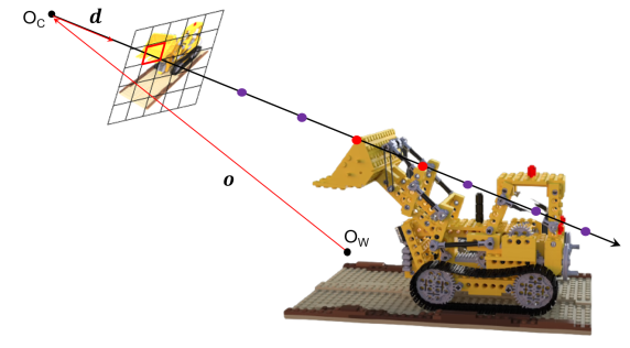
When NeRF uses the MLP to implicitly reconstruct a 3D scene, the inputs are poses of sampling points. NeRF aims to generate a 2D image in a new angle of view. To achieve this, we need to figure out how to obtain the poses of sampling points and how to use the reconstructed 3D densities and colors to get such a 2D image.

Ray marching is the solution used by NeRF. Assume that \boldsymbol{o}o represents the position of the camera origin O_cOc in the world coordinate system, and \boldsymbol{d}d represents the direction vector of a ray, and tt represents the distance traveling in the ray direction from O_cOc. After ray marching is used, each pixel of the 2D image corresponds to a ray, and any position on any ray can be represented as \boldsymbol{r}(t)=\boldsymbol{o}+t\boldsymbol{d}r(t)=o+td. You can obtain poses of the sampling points by sampling these rays (specifically, using random sampling and importance sampling described below). You can obtain the RGB values of 2D pixels by integrating the sampling points on these rays (specifically, using the volume rendering method described below).

4. Random Sampling and Importance Sampling

NeRF combines random sampling and importance sampling to sample rays generated by ray matching. This is because objects in the space are sparsely distributed and only a small area on a ray may take effect for final rendering. If uniform sampling is used, many sampling points are wasted, and it is difficult for the network to learn the distribution of the entire continuous space. Therefore, the coarse to fine principle is adopted to construct a coarse sampling network and a fine sampling network to better sample the space.

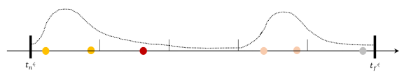
Random sampling: Evenly divides the rays from the near field to the far field ([t_n,t_f][tn,tf]) into N_cNc intervals, randomly selects a point in each interval, and inputs its spatial coordinate \boldsymbol{r}r and spatial angle of view \boldsymbol{d}d to the coarse sampling network to obtain the predicted RGB\sigmaRGBσ.

Importance sampling: Normalizes the weights w_iwi of all points on a ray output by the coarse sampling network (which will be described in the next section) as a probability density function (PDF) of the sampling intervals, randomly samples N_fNf points according to the PDF, combines the N_fNf points with the evenly sampled N_cNc points, and then inputs them to the fine sampling network.

NeRF calculates the mean squared errors (MSEs) between the rendering results (RGB values of 2D pixels) of the coarse/fine sampling networks and the ground truth, and uses the sum of the two errors as the total loss to train the two networks at the same time.

5. Volume Rendering

After the densities and RGB values of the sampling points are obtained, NeRF renders the 3D sampling values to a 2D plane by using the classic volume rendering technology in computer graphics. The specific principle is as follows.

The attenuation of light in the medium satisfies the following differential equation:

dL=-L\cdot \sigma \cdot dtdL=−L⋅σ⋅dt

LL is the luminous intensity and \sigmaσ is the attenuation coefficient. The solution is as follows:

L=L_0\cdot \exp(-\int{\sigma}dt)L=L0⋅exp(−∫σdt)

Assumptions:

(1) The color \boldsymbol{c}=[R,G,B]^Tc=[R,G,B]T of a spatial point is related to the line-of-sight direction \boldsymbol{d}d.

(2) The optical density \sigmaσ of a spatial point is irrelevant to the line-of-sight direction \boldsymbol{d}d.

This is because the color of an observed object is affected by the observation angle (such as the metal reflector), but the optical density is determined by the object material. The assumptions are also reflected in the NeRF network structure.

According to the attenuation equation and volume rendering principle of light in the medium, the rendering color of a pixel is represented as follows:

\boldsymbol{C}=\int_{t_{n}}^{t_{f}} T(t) \sigma(\boldsymbol{r}(t)) c(\boldsymbol{r}(t), \boldsymbol{d}) dtC=∫tntfT(t)σ(r(t))c(r(t),d)dt

T(t)=\exp(-\int_{t_n}^{t}{\sigma(\boldsymbol{r}(s))}ds)T(t)=exp(−∫tntσ(r(s))ds) represents the cumulative light transmittance within [t_n, t][tn, t], and \sigma(\boldsymbol{r}(t))dtσ(r(t))dt represents the luminous intensity attenuation rate within a distance from the microelement dtdt, which is equivalent to the reflectivity at \boldsymbol{r}(t)r(t).

Then, discretize the integral formula to make it suitable for computer processing. Select NN points along the ray. Within the interval length \delta_iδi represented by each point ii, \sigma, \mathbf{c}σ, and c are considered as constants, and the expression of the RGB values of 2D pixels obtained through rendering can be expressed as follows

\hat{C}(\mathbf{r})=\sum_{i=1}^{N}{T_i(1-\exp(-\sigma_i \delta_i))\mathbf{c_i}}C^(r)=i=1∑NTi(1−exp(−σiδi))ci

The cumulative light transmittance is T_i=\exp(-\sum_{j=1}^{i-1}\sigma_j \delta_j)Ti=exp(−∑j=1i−1σjδj).

The RGB values of 2D pixels obtained through volume rendering can be used to calculate the loss or generate the final 2D image in a new angle of view. At the same time, the following two parameters can also be obtained:

· \alpha_i=1-\exp(-\sigma_i \delta_i)αi=1−exp(−σiδi) is the opacity of the ii interval. Therefore, T_i=\prod_{j=1}^{i-1}{(1-\alpha_i)}Ti=∏j=1i−1(1−αi) is the cumulative transparency of the first (i–1i1) intervals.

· w_i=T_i\cdot \alpha_iwi=Ti⋅αi is the contribution rate of the color of the ii point to the rendered color, that is, the weight, which can be used to calculate the PDF of the coarse sampling network.

6. Overall NeRF Process

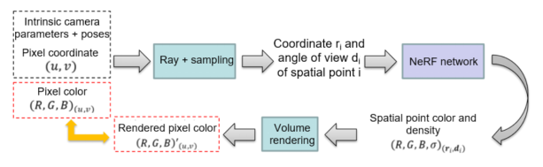
The following figure shows the NeRF process of synthesizing a scene in a new angle of view.

1. Input images with multiple angles of view (including pixel coordinates and colors), intrinsic camera parameters, poses, and other necessary data.

2. Use ray marching to generate rays and adopt random sampling and importance sampling to obtain the coordinates of spatial sampling points.

3. Input the coordinates of the spatial sampling points and the angle of view of each ray to NeRF with positional encoding to obtain the network prediction of the RGB\sigmaRGBσ value of each spatial point.

4. According to the RGB\sigmaRGBσ value of each spatial point, render the RGBRGB of the corresponding 2D pixel point of each ray by using volume rendering.

5. Perform MSE loss on the RGBRGB of pixel points obtained through prediction and rendering and the ground truth to train the neural network.

Code Process

Project website: will be released after the operators are optimized.

Program implementation environment: MindSpore 1.6.1 + CUDA 11.1.

Overall experiment process:

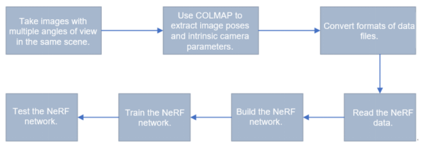
1. Data Preparation

In addition to images with multiple angles of view taken in the same scene, NeRF training also requires the intrinsic camera parameters and the pose of each image. The latter cannot be obtained through direct measurement. Therefore, certain algorithms are required.

COLMAP is a piece of general structure from motion (SfM) and multi-view stereo (MVS) software used to reconstruct point clouds. We use COLMAP to obtain the intrinsic camera parameters and the pose of each image, and estimate the depth range of camera imaging based on the coordinates of the 3D feature points to determine the far and near planes, that is, the boundaries.

Procedure:

1. Install COLMAP. Download it from the official website.

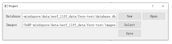
2. Open the software, choose File > New project, import the images folder, and create a database file in the directory where the folder is located.

3. Choose Processing > Feature extraction to extract feature points from the images.

4. Choose Processing > Feature matching to match feature points.

5. Choose Reconstruction > Start reconstruction to perform sparse reconstruction.

6. Choose Reconstruction > Dense reconstruction and click Undistortion to output the sparse reconstruction result, including the binary file containing information about the intrinsic camera parameters, image poses, and 3D feature points.

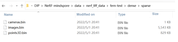
The data generated by COLMAP is a binary file. You need to save it as a poses_bounds.npy file to facilitate subsequent data loading. The procedure is as follows:

Execute the img2pose.py file. Before the execution, set the formal parameter to the directory where the dense folder is located.

After the execution, the pose_bounds.npy file is generated in the corresponding folder, and the data preprocessing is complete. The pose_bounds.npy file includes intrinsic camera parameters, the pose of each image (a transformation matrix from the camera coordinate system to the world coordinate system), and the imaging depth range of each image calculated based on 3D feature point information in the image.

In addition, the number of pixels of the original photographed images is too large to be calculated. Therefore, downsampling needs to be performed on the images in advance to reduce the calculation amount. Herein, 8x downsampling is used.

2. Model Building

2.1 Backbone Network Module

The first step is to build the backbone model.

Model inputs: high-dimensional vectors of spatial 3D coordinates after positional encoding.

Model outputs: predicted values at the corresponding 3D coordinates.

For details about the model architecture, see the principle section.

Pay attention to the initialization of model weights, which has a great impact on the convergence speed of training. Herein, the weights and offsets are evenly distributed in (-\sqrt{k},\sqrt{k})(−k,k), where k=1/\text{in-channels}k=1/in-channels. It has been tested that this initialization manner is helpful for NeRF convergence.

class LinearReLU(nn.Cell):

    def __init__(self, in_channels, out_channels):

        super().__init__()

        self.linear_relu = nn.SequentialCell([

            nn.Dense(in_channels, out_channels,

                     weight_init=Uniform(-math.sqrt(1. / in_channels)),

                     bias_init=Uniform(-math.sqrt(1. / in_channels))),

            nn.ReLU()

        ])



    def construct(self, x):

        return self.linear_relu(x)



    

class NeRF(nn.Cell):

    def __init__(self, D=8, W=256, input_ch=3, input_ch_views=3, skips=[4], use_viewdirs=False):

        super(NeRF, self).__init__()

        self.D = D

        self.W = W

        self.input_ch = input_ch

        self.input_ch_views = input_ch_views

        self.skips = skips

        self.use_viewdirs = use_viewdirs

        self.pts_layers = nn.SequentialCell(

            [LinearReLU(input_ch, W)] +

            [LinearReLU(W, W) if i not in self.skips else LinearReLU(W + input_ch, W)

             for i in range(D - 1)]

        )



        self.feature_layer = LinearReLU(W, W)

        if use_viewdirs:

            self.views_layer = LinearReLU(input_ch_views + W, W // 2)

        else:

            self.output_layer = LinearReLU(W, W // 2)



        self.sigma_layer = nn.SequentialCell([

            nn.Dense(W, 1,

                     weight_init=Uniform(-math.sqrt(1. / W)),

                     bias_init=Uniform(-math.sqrt(1. / W))) if use_viewdirs

            else nn.Dense(W // 2, 1,

                          weight_init=Uniform(-math.sqrt(1. / (W // 2))),

                          bias_init=Uniform(-math.sqrt(1. / (W // 2)))),

        ])

        self.rgb_layer = nn.SequentialCell(

            nn.Dense(W // 2, 3,

                     weight_init=Uniform(-math.sqrt(1. / (W // 2))),

                     bias_init=Uniform(-math.sqrt(1. / (W // 2)))),

            nn.Sigmoid()

        )



    def construct(self, x):

        pts, views = mnp.split(x, [self.input_ch], axis=-1)

        h = pts

        for i, l in enumerate(self.pts_layers):

            h = self.pts_layers(h)

            if i in self.skips:

                h = mnp.concatenate([pts, h], -1)



        if self.use_viewdirs:

            sigma = self.sigma_layer(h)

            feature = self.feature_layer(h)

            h = mnp.concatenate([feature, views], -1)

            h = self.views_layer(h)

            rgb = self.rgb_layer(h)



        else:

            h = self.feature_layer(h)

            h = self.output_layer(h)

            sigma = self.sigma_layer(h)

            rgb = self.rgb_layer(h)



        outputs = mnp.concatenate([rgb, sigma], -1)

        return outputs

2.2 Positional Encoding Module

Positional encoding needs to map the input 3D coordinates to a high dimension. Therefore, a list consisting of the \sin, \cossin, and cos functions needs to be constructed, which is traversed for every input. The output results are concatenated into the high dimension.

class Embedder: def __init__(self, **kwargs): self.kwargs = kwargs self.create_embedding_fn() def create_embedding_fn(self): embed_fns = [] d = self.kwargs['input_dims'] out_dim = 0 if self.kwargs['include_input']: embed_fns.append(lambda x: x) out_dim += d max_freq = self.kwargs['max_freq_log2'] N_freqs = self.kwargs['num_freqs'] if self.kwargs['log_sampling']: pow = ops.Pow() freq_bands = pow(2., mnp.linspace(0., max_freq, N_freqs)) else: freq_bands = mnp.linspace(2. ** 0., 2. ** max_freq, N_freqs) for freq in freq_bands: for p_fn in self.kwargs['periodic_fns']: embed_fns.append(lambda x, p_fn=p_fn, freq=freq: p_fn(x * freq)) out_dim += d self.embed_fns = embed_fns self.out_dim = out_dim def embed(self, inputs): return mnp.concatenate([fn(inputs) for fn in self.embed_fns], -1) def get_embedder(L): embed_kwargs = { 'include_input': True, 'input_dims': 3, 'max_freq_log2': L - 1, 'num_freqs': L, 'log_sampling': True, 'periodic_fns': [mnp.sin, mnp.cos], } embedder_obj = Embedder(**embed_kwargs) embed = lambda x, eo=embedder_obj: eo.embed(x) return embed, embedder_obj.out_dim

2.3 Loss Network

NeRF calculates the sum of two network losses as the total loss to optimize the two networks. Therefore, the NeRFWithLossCell class is required to connect the forward network to the loss function. The forward propagation process is complex and involves steps such as spatial sampling, positional encoding, neural network prediction, and volume rendering. These steps are also required in the test phase. Therefore, they are encapsulated into a function sample_and_render(). With only the ray information (rays), network information (net_kwargs), and training/test parameter settings (train_kwargs/test_kwargs) as the inputs, you can obtain the predicted RGB values of the pixels corresponding to each ray.

The properties of the class include the optimizer, network information, and psnr required for printing information. psnr is also a loss function, but it is not the optimization target and cannot be used as the output of construct. It can only be recorded as a property.

class NeRFWithLossCell(nn.Cell): def __init__(self, optimizer, net_coarse, net_fine, embed_fn_pts, embed_fn_views): super(NeRFWithLossCell, self).__init__() self.optimizer = optimizer self.net_coarse = net_coarse self.net_fine = net_fine self.embed_fn_pts = embed_fn_pts self.embed_fn_views = embed_fn_views self.net_kwargs = { 'net_coarse': self.net_coarse, 'net_fine': self.net_fine, 'embed_fn_pts': self.embed_fn_pts, 'embed_fn_views': self.embed_fn_views } self.psnr = None def construct(self, H, W, K, rays_batch, rgb, chunk=1024 * 32, c2w=None, ndc=True, near=0., far=1., use_viewdirs=False, **kwargs): # Data preparation: obtain the position, direction, near and far fields, and angle of view of each ray. rays = get_rays_info(H, W, K, rays_batch, c2w, ndc, near, far, use_viewdirs=True) # Sampling + rendering rets_coarse, rets_fine = sample_and_render(rays, **self.net_kwargs, **kwargs) # Loss calculation loss_coarse = img2mse(rets_coarse['rgb_map'], rgb) loss_fine = img2mse(rets_fine['rgb_map'], rgb) loss = loss_coarse + loss_fine self.psnr = mse2psnr(loss_coarse) return loss

2.4 Training Network

This class encapsulates the loss network and optimizer, and updates the network parameters using the optimizer in step-by-step mode.

class NeRFTrainOneStepCell(nn.TrainOneStepCell): def __init__(self, network, optimizer): super(NeRFTrainOneStepCell, self).__init__(network, optimizer) self.grad = ops.GradOperation(get_by_list=True) self.optimizer = optimizer def construct(self, H, W, K, rays_batch, rgb, **kwargs): weights = self.weights loss = self.network(H, W, K, rays_batch, rgb, **kwargs) grads = self.grad(self.network, weights)(H, W, K, rays_batch, rgb, **kwargs) return F.depend(loss, self.optimizer(grads))

3. Sampling

3.1 Coarse Sampling

Coarse sampling randomly samples evenly distributed segments along a ray. The inputs are the ray, number of sampling points, and other parameter settings. The outputs are the 3D coordinate pts of each sampling point, the distance z_vals of each sampling point in the -z direction, and the segmentation point z_splits in the -z direction.

def sample_coarse(rays, N_samples, perturb=1., lindisp=False, pytest=False): N_rays = rays.shape[0] rays_o, rays_d = rays[:, 0:3], rays[:, 3:6] near, far = rays[..., 6:7], rays[..., 7:8] t_vals = mnp.linspace(0, 1, N_samples + 1) if not lindisp: z_splits = near * (1. - t_vals) + far * t_vals else: z_splits = 1. / (1. / near * (1. - t_vals) + 1. / far * t_vals) z_splits = mnp.broadcast_to(z_splits, (N_rays, N_samples + 1)) if perturb > 0.: upper = z_splits[..., 1:] lower = z_splits[..., :-1] t_rand = np.random.rand(*list(upper.shape)) if pytest: np.random.seed(0) t_rand = np.random.rand(*list(z_splits.shape)) t_rand = Tensor(t_rand, dtype=ms.float32) z_vals = lower + (upper - lower) * t_rand else: z_vals = .5 * (z_splits[..., 1:] + z_splits[..., :-1]) pts = rays_o[..., None, :] + rays_d[..., None, :] * z_vals[..., :, None] return pts, z_vals, z_splits

3.2 Fine Sampling

Fine sampling uses the segmented weights obtained through coarse sampling as the PDF to sample data and then concatenates the fine and coarse sampling results to obtain fine sampling output. Herein, sample_pdf() is used for sampling based on the PDF, and main steps of program implementation are as follows:

1. According to the PDF, calculate the cumulative distribution function (CDF). It is also a piecewise linear function.

2. Within the [0, 1], sample the CDF values using uniform distribution.

3. Map the sampled CDF values back to coordinate values.

In step 3, we need to use the high-dimensional searchsorted operator to search for the index of coordinate values. However, the searchsorted operator of MindSpore supports only 1D inputs now and cannot handle this task. Therefore, we use the corresponding PyTorch operator temporarily.

def sample_pdf(bins, weights, N_samples, det=False, pytest=False): weights = weights + 1e-5 pdf = weights / mnp.sum(weights, -1, keepdims=True) cdf = mnp.cumsum(pdf, -1) cdf = mnp.concatenate([mnp.zeros_like(cdf[..., :1]), cdf], -1) if det: u = mnp.linspace(0., 1., N_samples) u = mnp.broadcast_to(u, tuple(cdf.shape[:-1]) + (N_samples,)) else: u = np.random.randn(*(list(cdf.shape[:-1]) + [N_samples])) u = Tensor(u, dtype=ms.float32) if pytest: np.random.seed(0) new_shape = list(cdf.shape[:-1]) + [N_samples] if det: u = np.linspace(0., 1., N_samples) u = np.broadcast_to(u, new_shape) else: u = np.random.rand(*new_shape) u = Tensor(u, dtype=ms.float32) cdf_tmp, u_tmp = torch.Tensor(cdf.asnumpy()), torch.Tensor(u.asnumpy()) inds = Tensor(torch.searchsorted(cdf_tmp, u_tmp, right=True).numpy()) below = ops.Cast()(mnp.stack([mnp.zeros_like(inds - 1), inds - 1], -1), ms.float32) below = ops.Cast()(below.max(axis=-1), ms.int32) above = ops.Cast()(mnp.stack([(cdf.shape[-1] - 1) * mnp.ones_like(inds), inds], -1), ms.float32) above = ops.Cast()(above.min(axis=-1), ms.int32) inds_g = mnp.stack([below, above], -1) matched_shape = (inds_g.shape[0], inds_g.shape[1], cdf.shape[-1]) cdf_g = ops.GatherD()(mnp.broadcast_to(cdf.expand_dims(1), matched_shape), 2, inds_g) bins_g = ops.GatherD()(mnp.broadcast_to(bins.expand_dims(1), matched_shape), 2, inds_g) denom = (cdf_g[..., 1] - cdf_g[..., 0]) denom = mnp.where(denom < 1e-5, mnp.ones_like(denom), denom) t = (u - cdf_g[..., 0]) / denom samples = bins_g[..., 0] + t * (bins_g[..., 1] - bins_g[..., 0]) return samples

4. Ray Acquisition

get_rays() uses the image size [H,W][H,W], intrinsic camera parameter matrix KK, and camera pose c2wc2w to calculate the position ray rays_o and direction ray rays_d of each pixel in the world coordinate system. The OpenGL coordinate system is used, in which the positive xx is to your right, the positive yy is up, and the positive zz is backwards. rays_d is normalized in the -z direction, that is, the orientation of the camera when the image was taken. During coarse sampling and fine sampling, all rays in different directions are sampled based on their distances in the -z direction.

get_rays_info() is used to concatenate all information about rays into a rays tensor for subsequent invocation. The ray information includes:

1. Position vector rays_o

2. Direction vector rays_d

3. Near field (lower limit of integration during volume rendering)

4. Far field (upper limit of integration during volume rendering)

5. United view angle vector view_dir

def get_rays(H, W, K, c2w): i, j = mnp.meshgrid(mnp.linspace(0, W - 1, W), mnp.linspace(0, H - 1, H), indexing='xy') dirs = mnp.stack([(i - K[0][2]) / K[0][0], -(j - K[1][2]) / K[1][1], -mnp.ones_like(i)], -1) c2w = Tensor(c2w) rays_d = mnp.sum(dirs[..., None, :] * c2w[:3, :3], -1) rays_o = ops.BroadcastTo(rays_d.shape)(c2w[:3, -1]) return rays_o, rays_d def get_rays_info(H, W, K, rays_batch=None, c2w=None, ndc=True, near=0, far=1, use_viewdirs=True): if c2w is not None: rays_o, rays_d = get_rays(H, W, K, c2w) else: rays_o, rays_d = rays_batch if use_viewdirs: viewdirs = rays_d viewdirs = viewdirs / mnp.norm(viewdirs, axis=-1, keepdims=True) viewdirs = mnp.reshape(viewdirs, [-1, 3]) if ndc: rays_o, rays_d = ndc_rays(H, W, K[0][0], 1., rays_o, rays_d) rays_o = mnp.reshape(rays_o, [-1, 3]) rays_d = mnp.reshape(rays_d, [-1, 3]) near, far = near * mnp.ones_like(rays_d[..., :1]), far * mnp.ones_like(rays_d[..., :1]) rays = mnp.concatenate([rays_o, rays_d, near, far], -1) if use_viewdirs: rays = mnp.concatenate([rays, viewdirs], -1) return rays

5. Rendering

Based on RGB\sigmaRGBσ of each spatial sampling point output by the network, calculate the RGB value of the 2D pixel point corresponding to a ray by using the volume rendering formula. This function is the main framework of NeRF forward propagation. The main process is as follows:

1. Perform coarse sampling on the ray data.

2. Concatenate the sampling point coordinate pts_coarse obtained through coarse sampling with the ray direction vector views_coarse, and input them to the coarse sampling network. After positional encoding and neural network forward propagation, the predicted value raw_coarse of RGB\sigmaRGBσ of the spatial sampling point can be obtained. views_coarse is the unit vector of rays_d, which eliminates the impact of different vector magnitudes.

3. Input raw_coarse to the volume rendering function render() to obtain the return value ret_coarse, a dictionary that contains all rendered results, including the weights rets_coarse['weights'] of coarse sampling points.

4. Perform fine sampling based on the weights of the sampling points on the coarse sampling network and the sampling segments.

5. Concatenate the spatial sampling point coordinate pts_fine obtained through fine sampling with the ray direction vector views_fine, and input them to the fine sampling network. After positional encoding and neural network forward propagation, the predicted value raw_fine of RGB\sigmaRGBσ of the spatial sampling point can be obtained.

6. Input raw_fine to the volume rendering function render() to obtain the return value ret_fine, which also includes all rendering results.

7. Output the return values rets_coarse and rets_fine of the coarse sampling network and fine sampling network.

def sample_and_render(rays, net_coarse=None, net_fine=None, embed_fn_pts=None, embed_fn_views=None, N_coarse=64, N_fine=64, perturb=1., lindisp=False, pytest=False, raw_noise_std=0., white_bkgd=False): # Data preparation rays_d = rays[..., 3: 6] views = rays[:, -3:] if rays.shape[-1] > 8 else None # Coarse sampling pts_coarse, z_coarse, z_splits = sample_coarse(rays, N_coarse, perturb, lindisp, pytest) views_coarse = mnp.broadcast_to(views[..., None, :], pts_coarse.shape) sh = pts_coarse.shape # Positional encoding of the coarse sampling network pts_embeded_coarse = embed_fn_pts(pts_coarse.reshape([-1, 3])) views_coarse_embeded = embed_fn_views(views_coarse.reshape([-1, 3])) # Input of the coarse sampling network and output after rendering net_coarse_input = mnp.concatenate([pts_embeded_coarse, views_coarse_embeded], -1) raw_coarse = net_coarse(net_coarse_input).reshape(list(sh[:-1]) + [4]) rets_coarse = render(raw_coarse, z_coarse, rays_d, raw_noise_std, white_bkgd, pytest) # Fine sampling weights = rets_coarse['weights'] pts_fine, z_fine = sample_fine(rays, z_coarse, z_splits, weights, N_fine, perturb, pytest) views_fine = mnp.broadcast_to(views[..., None, :], pts_fine.shape) sh = pts_fine.shape # Positional encoding of the fine sampling network pts_embeded_fine = embed_fn_pts(pts_fine.reshape([-1, 3])) views_embeded_fine = embed_fn_views(views_fine.reshape([-1, 3])) # Input of the fine sampling network and output after rendering net_fine_input = mnp.concatenate([pts_embeded_fine, views_embeded_fine], -1) raw_fine = net_fine(net_fine_input).reshape(list(sh[:-1]) + [4]) rets_fine = render(raw_fine, z_fine, rays_d, raw_noise_std, white_bkgd, pytest) return rets_coarse, rets_fine

6. Main Function

The tasks of the main function are as follows:

1. Load images, poses, and intrinsic parameters, divide them into batches, and disorder them.

2. Use create_nerf() to create a NeRF model. The return values include the dictionary net_kwargs composed of network instances, training parameters train_kwargs, test parameters test_kwargs and, optimizer.

3. Build the loss network net_with_loss and load the previously saved training parameters.

4. Build the training network train_net.

5. Iteratively optimize train_net.

6. Save the training parameters and the rendered video.

Invoke the training network during training. train_net(H, W, K, batch_rays, target_s, **train_kwargs)

References

[1] Mildenhall, B., Srinivasan, P.P., Tancik, M., Barron, J.T., Ramamoorthi, R., Ng, R. (2020). NeRF: Representing Scenes as Neural Radiance Fields for View Synthesis. In: Vedaldi, A., Bischof, H., Brox, T., Frahm, JM. (eds) Computer Vision – ECCV 2020. ECCV 2020.

[2] Official Implementation of the NeRF Paper: https://github.com/bmild/nerf

[3] Pytorch Implementation of NeRF: https://github.com/yenchenlin/nerf-pytorch

[4] MindSpore 1.6 API: https://www.mindspore.cn/docs/en/r1.6/index.html