MindSpore Made Easy Deep Learning Series: Optimization Algorithm – Exponentially Weighted Average

Today, we'll continue our learning on the exponentially weighted average (EWA), a statistical measure used by optimization algorithms.

Basic Principles

The EWA is also known as the exponentially weighted moving average (EWMA). With its help, we can calculate local average values and describe the change trend of data. This blog takes the case of temperature as an example.

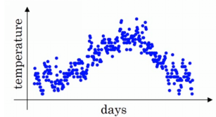
This figure shows the relationship between time and temperature. The horizontal axis indicates a day in a year, and the vertical axis indicates the temperature of the day. The temperatures in January and December are lower than those in June and July.

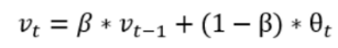
The local average (moving average) of temperatures is used to describe the temperature change trend. The formula is as follows:

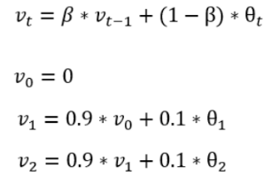
v__i indicates the local average, namely the temperature of a certain day. In calculation, v__t can be considered as the daily temperature of 1/((1 – β)).

Here, we select three typical cases for further description:

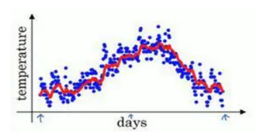
1. Assume the value of β is 0.9. The temperature trend of 10 days is calculated, as shown in the red curve in the following figure.

2. Assume that the value of β is close to 1, such as 0.98. 1/(1 – 0.98) = 50. The temperature of the past 50 days is averaged, as shown by the green line in the figure.

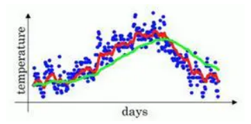
Then a flatter curve is obtained because the temperatures of several more days are averaged. However, the curve is further moved to the right in this way. In other words, when β = 0.98, too much weight is added to the previous day, but only a weight of 0.02 is given to the current day. Therefore, when β is greater, the EWA takes more time to adapt.

3. Set β to 0.5 to average the temperatures of two days. The yellow line in the following figure shows the local temperature average.

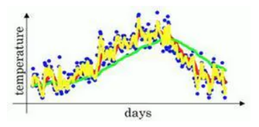
As the averaged data is too small (only the temperatures of two days are averaged), the obtained curve has more noise in it. Though abnormal values may exist, this curve can adapt to the temperature change in a shorter period.

Further Research

It is not difficult to find that the key equation for calculating the EWA is as follows:

When β = 0.9:

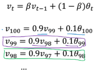
In this way, the equation can be expanded as such:

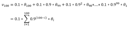
Based on the preceding formula, we can get an exponential decay function: 0.1, 0.1 x 0.9, 0.1 x (0.9)2, ...

It can also explain why the temperatures are averaged for only 10 days when β = 0.9.

ε = 1 – β = 1 – 0.9 = 0.1. When (1 – ε)1/ε = 1/e, namely (0.9)10 = 1/e (e is the natural logarithm), the weight decreases to 1/e of the maximum weight, and the number of averaged days is 1/ε=1/(1 – β).

In general, to obtain the average value of the local temperatures in 10 days, we need to calculate with the temperatures in the latest 10 days. However, with the EWA, we only need to know the previous weighted average value. In this way, it speeds up calculation while occupying little memory but compromising some accuracy.

Deviation Correction

Deviation correction is here to address this challenge. It can improve the accuracy of the EWA, mainly for the average values in the early stage.

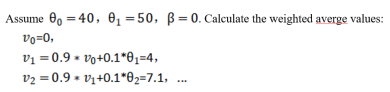
Through calculation, we can find that the weighted average values in the early stage deviate a lot, and that's why deviation correction is introduced.

v__t /1 – β_t_ is used to correct the error of the EWA. However, as t increases, 1 – β_t_ becomes closer to 1. As a result, the deviation correction has little impact on the average values in the late stage.

Conclusion

For the EWA, different (β) parameters lead to different results. By applying a certain value, we may achieve the best outcome and can better average data.

That's all about today's learning. If you have any suggestions, feel free to contact us.