MindSpore Made Easy Deep Learning Series - Dropout

In addition to L2 regularization, another powerful regularization technique is dropout.

1.1 How Dropout Works

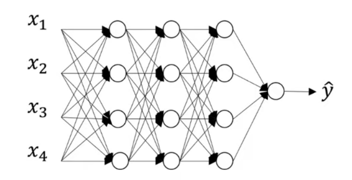
Assume the neural network in the figure is overfitting. In this case, dropout can play the magic. To use dropout, for each layer of the network, set a probability of eliminating a node in the network. Assume that for each layer, we toss a coin for each node and set a 0.5 chance of keeping each node, and of course, a 0.5 chance of eliminating each node. Then, we can obtain a much smaller network with fewer nodes to be trained on one sample using back propagation.

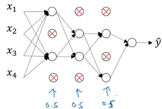
For a different sample, set the probability for each node by tossing the coins again, and keep a different set of nodes. Each training sample is used to train one of these reduced networks.

Then, let's look at how to implement dropout.

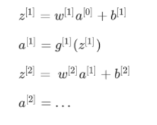
The most common method is inverted dropout. Take a network with 3 layers as an example, where we want to implement dropout in a single layer.

First, set the vector d. d[3] denotes the dropout vector for layer 3.

d3 = np.random.rand(a3.shape[0],a3.shape[1])

Then, the elements of d[3] will be compared with a certain value called keep-prob. keep-prob is a specific number. In the previous coin-tossing example, keep-prob is 0.5. In this example, set keep-prob to 0.8, which is the probability of keeping a hidden unit. In other words, the probability of eliminating any hidden unit is 0.2. d[3] is a matrix. For each sample and each hidden unit, there is a 0.8 chance that the corresponding element of d[3] being 1 and a 0.2 chance it being 0.

Next, we obtain the activation function a[3] from the third layer. a[3] is equal to the old a[3] times d[3] (a3 =np.multiply(a3,d3)). In this way, for every element of d[3] that is 0 (there is a 0.2 chance of each element being 0), this multiply operation ends up zeroing out the corresponding element of a[3]. In Python, d[3] is a Boolean array whose values are true and false, which are interpreted as 1s and 0s.

Finally, scale out a[3] by dividing it by 0.8, that is, the keep-prob parameter.

So, what is the purpose of this final step? Assumed that there are 50 units, or 50 neurons, in the third hidden layer. Then a[3] is 50 x 1 dimensional, or with factorization, 50 x m dimensional. If probabilities of keeping and deleting the units are 80% and 20% respectively, on average, 10 (50 x 20%) units are zeroed out. Since 20% of the elements of a[3] are zeroed out, in order not to reduce the expected value of z[4], which equals to w[4]a[3], divide a[3] by 0.8. This will correct the 20% reduction, and the expected value of a[3] does not change.

If keep-prop is set to 1, dropout does not exist because all nodes are kept. The inverted dropout technique ensures that the expected value of a[3] remains the same by dividing a[3] by keep-prob.

Practice has proved that at test time when we evaluate a neural network, inverted dropout makes evaluation easier because it has less of a scaling problem.

Generally, if multiple passes are made through the same training set, the gradient varies with each pass, and different hidden units are zeroed out. However, sometimes this is not the case. So, on the first iteration of gradient descent, some hidden units should be zeroed out; on the second iteration where the training set is gone through a second time, a different pattern of hidden units should be zeroed out. The vector d for the third layer (d[3]) decides which units are zeroed out.

At test time, we have X (X=a[0]), on which we want to make a prediction using the standard notation.

And so on, until we get the last layer and make a prediction y.

Notice that at test time, dropout is not used to prevent the prediction from being interfered. Theoretically, you can run the prediction process many times with different hidden units randomly dropped out and then average across them. However, this calculation is inefficient and gives roughly the same result as that of the procedure above.

In inverted dropout, the purpose of dividing a[3] by keep-prob is to ensure that even dropout is not implemented to the scaling at test time, the expected values of the activations don't change, avoiding the need to add an extra scaling parameter. This is different at training time.

1.2 Understanding Dropout

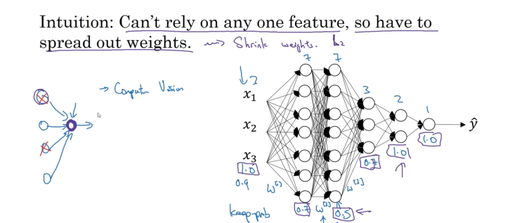
Intuitively speaking, a unit (the circle in purple) cannot rely on any one feature because any one input of the unit may be eliminated at random. Therefore, the unit spreads out its weight to each of the four inputs. By spreading out the weights, dropout tends to have an effect of shrinking the squared norm of the weights and helps prevent overfitting, which is similar to L2 regularization. However, the L2 penalty on different weights is different, depending on the scale of the activations being multiplied to.

To summarize, dropout has a similar effect to L2 regularization, only that L2 regularization applied to different weights can be different and more adaptive to different scales of inputs.

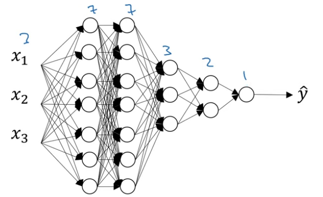
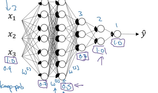
One more detail for dropout implementation is the value of keep-prob. Here's a network with three input features. One of the parameters to be decided is keep-prob, which is the chance to keeping a unit in each layer. It is feasible to vary keep-prob by layer. For the first layer, the size of the weight matrix W[1] is 7 x 3; the size of the second weight matrix W[2] is 7 x 7; the size of W[3] is 3 x 7, and so on. W[2] is the biggest weight matrix because layer 2 has the largest set of parameters. To prevent overfitting of W[2], set keep-prob to a relatively small value, for example, 0.5. For other layers where overfitting is less likely to occur, the value of keep-prob can be set bigger, for example, 0.7.

To summarize, if you are more worried about some layers overfitting than others, you can set a lower keep-prob for them. The downside is that this results in more hyperparameters to search for during cross-validation. One alternative is to apply dropout to certain layers. A layer to which dropout is applied has only one hyperparameter, that is, keep-prob.

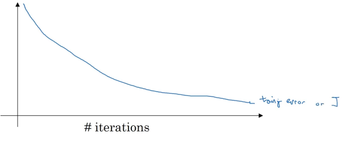
One big downside of dropout is that the cost function J is no longer well defined. On every iteration, some nodes are randomly eliminated. This makes it harder to double check the performance of gradient descent. A well-defined cost function J goes downhill on every iteration. Since the cost function we are optimizing is not well-defined or hard to calculate, we lose the debugging tool by plotting a graph like this. In this case, you can turn off dropout, set keep-prob to 1 to make sure that the J function is monotonically decreasing, and then turn on dropout.

1.3 Other Regularization Methods

In addition to L2 regularization and dropout, there are a few other techniques to reduce overfitting in neural networks.

1. Data Augmentation

Assume that we have a dog classifier that is overfitting. Getting more training data can help but can also be expensive. Sometimes it is impossible to get more data. However, you can augment the training set by flipping the images horizontally, which nearly doubles the size of the training set. The training set now might be a bit redundant and not as good as a set of brand new independent images, but it prevents the need to pay the expense of collecting more images of dogs. Other than flipping the images, you can also randomly crop the images.

2. Early Stopping

When running gradient descent, you can plot either the training error (0-1 classification error on the training set) or the cost function J you are optimizing, which should decrease monotonically as the figure below.

As you train, you want the training error and cost function J to decrease. To implement early stopping, plot both training error and dev set error, which can be a classification error, cost function, logistic loss, or log loss on the dev set. You will find that the dev set error usually goes down for a while and then increase from a certain point.

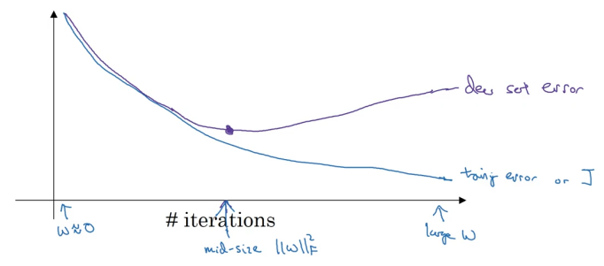
When you have not run many iterations for the neural network, the parameters W will be close to zero. This is because with random initialization, W is probably initialized to small random values. As you run iterations, W gets bigger and bigger. By stopping halfway, you get a mid-sized Frobenius norm. Similar to L2 regularization, picking a neural network with a smaller norm for W will reduce overfitting. Early stopping refers to the process of stopping training early.