Idea Sharing (35): New AI4Science Directions in Quantum, Atomistic, and Continuum Systems

Advancements of artificial intelligence (AI) are fueling a new paradigm for scientific discoveries. AI has begun to revolutionize the field of natural sciences by enhancing, speeding up, and facilitating our comprehension of natural phenomena across various spatial and temporal scales. This has led to the emergence of a new research field called AI for Science or AI4Science. The paper Artificial Intelligence for Science in Quantum, Atomistic, and Continuum Systems co-authored by over 60 individuals was recently published. It offers a detailed technical overview of a specific subfield of AI4Science, focusing on the application of AI to quantum, atomistic, and continuum systems. And this blog extracts technical principles of the paper and simply introduces how to construct an equivariant model through symmetry transformations.

1. Introduction

In 1929, Paul Adrien Maurice Dirac, a quantum physicist pointed out that "The underlying physical laws necessary for the mathematical theory of a large part of physics and the whole of chemistry are thus completely known, and the difficulty is only that the exact application of these laws leads to equations much too complicated to be soluble." This is true from the Schrödinger's equation in quantum physics to the Navier-Stokes equations in fluid mechanics. Fortunately, deep learning methods are able to accelerate the computing of solutions for these equations. Specifically, results generated by conventional simulation methods can be used as data to train deep learning models. Once trained, these models can make predictions at a speed that is much faster than conventional methods.

In other areas such as biology, the underlying biophysical processes are not fully understood and may not eventually be described by mathematical equations. In these cases, data generated by experiments may be used to train deep learning models. For example, protein prediction models, such as AlphaFold, RoseTTAFold, and ESMFold, trained by using 3D structures obtained by experiments, can achieve an accuracy comparable to experimental results in terms of computational predictions of protein 3D structures.

1.1 Scientific Areas

Based on the spatial and temporal scales at which the physical world is modeled, the following figure provides an integrative overview of research areas in AI4Science.

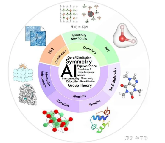
Small scale: Quantum mechanics uses wave functions to investigate physical occurrences at the most minute length scales, which describe the complete dynamics of quantum systems. Typically, wave functions are derived by resolving the Schrödinger equation. This, however, involves exponential complexity. Density functional theory (DFT) and ab initio quantum chemistry methods are first principles widely used in practice to calculate electronic structures and physical properties of molecules and materials and to further derive other properties, including electronic, mechanical, optical, magnetic, and catalytic properties of molecules and solids. However, these methods are computationally expensive, restricting their application to only small systems (about 1,000 atoms). And AI models can exactly help improve speed and accuracy.

Medium scale: A small molecule typically has tens to hundreds of atoms and plays an important role in regulatory and signal transmission in many chemical and biological processes. Protein is a macromolecule consisting of one or more amino acid chains. Amino acid sequences are believed to determine protein structures, which in turn determine their functions. Materials science studies the relationship of processing, structure, and performance of materials. And molecular interaction studies how molecules interact with each other to implement physical and biological functions, such as ligand-receptor and molecule-material interactions. In these fields, AI has made much progress in molecular characterization and generation, molecular dynamics, protein structure prediction and design, material property prediction, and structure generation.

Large scale: Continuous mechanics uses partial differential equations (PDEs) to represent physical phenomena that progress over time and space at the macroscopic scale, including fluid flows, heat transfer, and electromagnetic waves. AI methods have provided solutions to problems such as improving computing efficiency, generalization, and multi-resolution analysis.

1.2 Technical Areas of AI

The following presents some common technical challenges that exist in multiple fields in AI4Science.

Symmetry: Symmetries are very strong inductive biases, and a key challenge of AI4Science is how to effectively integrate symmetries in AI models.

Interpretability: Interpretability is critical to understanding the laws of physical worlds in AI4Science.

Out-of-distribution (OOD) generalization and causality: To avoid generating training data for each different setting, causal factors capable of OOD generalization need to be identified.

Foundation and large language models: Foundations models involved in natural language processing (NLP) tasks are pre-trained under self-supervised or generalizable supervision, allowing various downstream tasks to be performed in zero-shot or few-shot mode. The paper describes how this paradigm accelerates discoveries in AI4Science.

Uncertainty quantification (UQ): It studies how to guarantee robust decision-making under data and model uncertainties.

Education: To facilitate learning and education, the paper lists the resources that the author considers useful and provides views on how the community can better promote the integration of AI with science and education.

2. Symmetries, Equivariance, and Theory

In many scientific problems, an object of interest is usually located in a 3D space, and any mathematical representation of the object depends on a reference coordinate system, making representations coordinate-dependent. However, there is no coordinate system in nature, so representations independent of the coordinate system are required. Therefore, one of the key challenges of AI4Science is how to achieve invariance or equivariance under coordinate system transformations.

2.1 Overview

Symmetries refer to attributes of a physical phenomenon remain unchanged under a transformation such as coordinate transformation. If certain symmetries exist in the system, the predicted target is naturally invariant or equivariant to the corresponding symmetry transformation. For example, when energies of 3D molecular structures are predicted, the predicted value remains unchanged even if the 3D molecule is translated or rotated. An optional strategy to achieve symmetry-aware learning is to use data augmentation during supervised learning. Specifically, random symmetry transformations are performed on input data and labels to force the model to output approximate equivariant predictions. However, this comes with many drawbacks. First, considering the additional degree of freedom for selecting a coordinate system, the model needs a larger capacity to represent a simple mode originally in a fixed coordinate system. Second, many symmetry transformations, such as translation, can produce an infinite number of equivariant samples, which makes it difficult for limited data augmentation to fully reflect the symmetries in the data. Third, in some cases, a very deep model needs to be built to achieve a good prediction effect. If each layer of the model cannot maintain equivariance, it will be difficult for the model to output equivariant predictions. Finally yet importantly, for scientific issues such as molecular modeling, it is critical to provide a robust prediction under symmetry transformations so that machine learning can be used in a reliable manner.

Given these disadvantages of data augmentation, more and more studies have focused on designing machine learning models that meet symmetry requirements. With symmetry-adapted architecture, models can focus on learning target prediction tasks without data augmentation.

2.2 Equivariance under Discrete Symmetry Transformations

In this part, the paper presents an example of maintaining equivariance under discrete symmetry transformations in AI models. This example simulates the mapping of a scalar fluid field in a 2D space at the current time step to the next time step. When the input fluid field is rotated by 90°, 180°, or 270°, the output fluid field is rotated accordingly. The mathematical expression is as follows:

f represents a fluid field mapping function, and R represents a discrete rotation transformation. The equivariant group convolutional neural networks (G-CNNs) were proposed to better achieve equivariance under symmetry transformations. One of the simplest solutions is the lifting convolution:

It performs convolutions with kernels rotated by every angle in α to generate several feature maps, and these feature maps are stacked at the rotation degree α. Then, it applies a pooling operation over α-axis. As such, the output rotates accordingly when the input X rotates.

Due to pooling operations, G-CNNs maintain equivariant lines which do not cannot carry direction information. As a result, G-CNNs typically adopt the structure shown in the following figure.

The typical architecture starts with a lifting convolution, which, as explained above, is followed by multiple equivariant group convolution layers. The final layer is a pooling layer that operates over the α-axis. In this way, intermediate feature layers can better detect patterns of features in their relative positions and orientations. The equivariance of intermediate feature layers refers to the fact that these layers rotate in correspondence with rotation transformations, with the sequence of the rotation dimension also being rotated. Rotation properties of a convolution kernel in a group convolution layer also enable an output feature map to maintain this equivariant feature.

2.3-2.5 Equivariant Model Construction of 3D Continuous Transformations

For many scientific problems, we focus on continuous transformations in a 3D space, for instance, translations and rotations of chemical compounds. Accordingly, vectors formed by predicted molecular properties also rotate. These consecutive rotations R and translations t form elements in SE(3) (SE stands for the special Euclidean group in a 3D space), and these transformations can be represented as transformation matrices in vector spaces. Transformation matrices in different vector spaces may be different, but all these vector spaces can be decomposed into mutually independent subvector spaces. Each subspace has a same transformation rule, that is, vectors generated after all transformation elements in the group are applied to vectors in the subspace still exist in this subspace. Therefore, transformation elements in the group can be represented by an irreducible transformation matrix in the subspace. For example, scalars such as total energy and band gaps remain unchanged under actions of elements in SE(3), and the transformation matrix is represented as D^0(R)=1. However, the force field rotates with the transformation matrix being represented as D^1(R)=R. In a higher-dimensional vector space, D^l(R) represents a (2l+1)-dimensional array. These transformation matrices D^l(R) are referred to as l-order Wigner-D matrix of R, and corresponding subvector spaces become l-order irreducible and unchanged subspaces of SE(3), where vectors are referred to as l-order equivariant vectors. In translations, these vectors always remain unchanged, because their properties are only associated with relative positions.

Generally, spherical harmonics are used to map 3D geometric information to the features in the invariant subspace of SE(3). Y^l, a set of spherical harmonics, maps an input 3D vector to a (2l+1)-dimensional vector representing the coefficient of (2l+1) spherical harmonics bases. As shown in the following figure, because only a limited number of bases are used, the delta function on the sphere represented by the 3D vector is expanded to some extent.

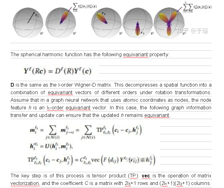
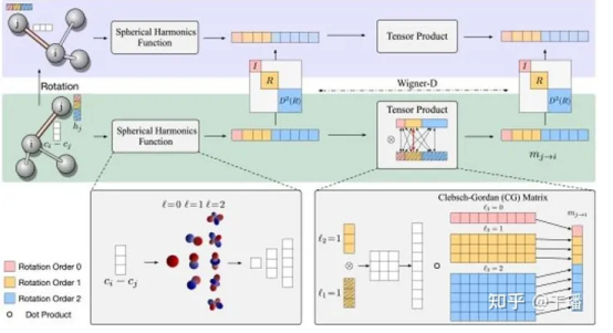
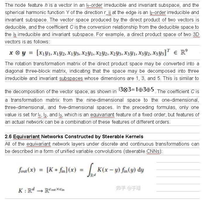
x and y are spatial coordinates, f_in(y) represents an input feature vector at the coordinate y, f_out(x) represents an output feature vector at the coordinate x, and K is transformation from an input feature space to an output feature space. Convolution operations ensure translation equivariance. However, to ensure equivariance under other spatial affine transformations, the convolution kernel K needs to meet the following symmetry constraint:

g is the transformation in a spatial transformation group, and ρ_in and ρ_out are representations (transformation matrices) of the transformation in input and output feature spaces, respectively.

This is all about theories related to symmetries and equivariance in the paper. If you are interested in applications in different domains, consult the subsequent chapters.

References:

[1] Xuan Zhang, Limei Wang, Jacob Helwig, et al. 2023. Artificial Intelligence for Science in Quantum, Atomistic, and Continuum Systems. arXiv: https://arxiv.org/abs/2307.08423

[2] Taco Cohen and Max Welling. 2016. Group Equivariant Convolutional Networks. In International Conference on Machine Learning. PMLR, 48:2990–2999.

[3] Nathaniel Thomas, Tess Smidt, Steven Kearnes, et al. 2018. Tensor field networks: Rotation-and translation-equivariant neural networks for 3d point clouds. arXiv: https://arxiv.org/abs/1802.08219

Maurice Weiler, Mario Geiger, Max Welling, et al. 2018. 3D Steerable CNNs: Learning Rotationally Equivariant Features in Volumetric Data. In Advances in Neural Information Processing Systems