Idea Sharing (30): FuXi Model

Overview

Since Pangu-Weather[1] unprecedentedly outperformed the conventional numerical methods in terms of medium- and long-term weather forecast accuracy, the industry has begun to explore the potential of meteorology foundation models. For example, GraphCast[2] based on graph neural networks has achieved high forecast accuracy within 10 days on assimilation data in ERA5. The FuXi foundation model[3] introduced in this blog is launched by the Artificial Intelligence Innovation and Incubation Institute of Fudan University. The model was developed based on data of 39 years from the ECMWF ERA5 reanalysis dataset. Using a cascade architecture, it can provide 15-day global forecast with a time resolution of 6 hours and spatial resolution of 0.25°. In the performance evaluation of latitude weighted root-mean-square error (RMSE) and anomaly correlation coefficient (ACC), the 15-day forecast of the model is comparable with the forecast result of ECMWF ensemble average (EM) for the first time.

Background

ECMWF's high-resolution endoluminal sonography (HRES) is considered to be one of the most accurate weather forecast models in the world. With a horizontal resolution of 0.1° and 137 vertical levels, it can provide a 10-day forecast. However, weather forecasts are inherently uncertain for the following reasons:

1. Limited resolution: The accuracy of weather forecast is affected by the resolution of the NWP model. As the resolution is low, the model may not fully capture weather phenomena at a smaller scale.

2. Physical process approximation: The NWP model relies on parametrization methods to represent complex physical processes that occur at scales below the model resolution, which introduce uncertainties.

3. Initially small errors will be magnified with time, resulting in significant forecast differences.

4. Chaotic characteristics of the atmosphere: Weather is a chaotic system. Tiny changes may have significant effects over time. This sensitivity to initial conditions increases the uncertainty.

5. Increase in forecast lead time: The longer the forecast lead time, the greater the uncertainty. This is due to the cumulative effect of various uncertainties and errors.

Weather centers such as ECMWF run an Ensemble Prediction System (EPS) to address uncertainties. The EPS of ECMWF includes multiple forecasts, which vary slightly in initial conditions and physical parametrization. By running these ensemble members, you can evaluate the range of possible results and estimate the forecast uncertainties.

Despite the benefits of ensemble prediction, the calculation cost is high because multiple simulations with perturbation conditions need to be run. In recent years, more and more efforts have been made to replace conventional NWP models with machine learning models for weather forecast. Machine learning–based weather forecast systems have several advantages over NWP models, including higher speeds and possible higher accuracies provided by training using reanalysis data. To facilitate comparison between different machine learning models, WeatherBench is introduced to evaluate mid-term weather forecasts (3 to 5 days). WeatherBench regridizes ERA5 and then analyzes the data[4]. The 0.25° resolution is converted into 5.625°, 2.8125°, and 1.40625° resolutions.

The FuXi model is an autoregressive model. It uses the weather parameters of the first two time steps as the input to predict the weather parameters of the next time step. The time step of the model is 6 hours, and weather forecasts with different lead times are generated through iteration. Due to the lack of physical constraints in pure data-driven machine learning models, cumulative errors and unrealistic forecasts may occur during long-term forecasts. To address this challenge, the multi-step loss of autoregression is introduced, which is similar to the cost function of the 4D-Var method, to effectively reduce the error of long-term forecasts. However, increasing the number of autoregressive steps results in reduced accuracy of short-term forecasts and requires more memory and computing resources.

During iterative forecasting, error accumulation is inevitable as the lead time increases. In addition, a single model cannot always give the best performance when the lead time changes. In order to strike a balance between short- and long-term forecasts, a cascade model architecture is proposed. The cascaded model uses the pre-trained FuXi model and optimizes and fine-tunes 5-day forecast time windows, namely FuXi-Short (0-5 days), FuXi-Medium (5-10 days), and FuXi-Long (10-15 days).

Model Architecture

The basic FuXi model architecture consists of three main components: cube embedding, U-Transformer, and a fully connected (FC) layer, as shown in the following figure. The input data combines the upper-air and surface variables, and creates a data cube with dimensions of 2 × 70 × 721 × 1440, taking two time steps as a step.

The dimensionality of high-dimensional input data is reduced through joint space-time cube embedding and converted into C × 180 × 360. The main purpose of cube embedding is to reduce the temporal and spatial dimensionality of input data and reduce redundant information. Subsequently, U-Transformer processes the embedded data and uses a simple FC layer for forecast. The output is initially reshaped to 70 × 720 × 1440.

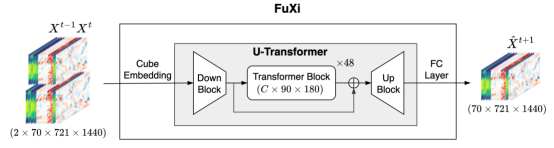
Figure 1 Overall architecture of the FuXi model

Cube Embedding

To reduce the spatial and temporal dimensionality of the input data and speed up the training process, cube embedding is applied. A similar method, called patch embedding, is also used in the Pangu-Weather model. Patch embedding divides an image into N × N patches. Each patch is transformed into a feature vector.

Specifically, a three-dimensional (3D) convolution layer is used in cube embedding with a convolution kernel and stride of 2 × 4 × 4 (equivalent to T/2 × H/2 × W/2). The number of output channels is C. After embedding, layer normalization (LayerNorm) is used to improve the stability of training. The dimensions of the finally obtained data cube are C × 180 × 360.

U-Transformer

The U-Transformer includes a downsampling and an upsampling block from the U-Net model. The downsampling block is called Down Block in the figure. It reduces the data dimensionality to C × 90 × 180, minimizing computational and memory requirements for self-attention calculation. The Down Block consists of a 3 × 3 2-dimensional (2D) convolution layer with a stride of 2 and a residual block. The residual block has two 3 × 3 convolution layers, followed by a group normalization (GN) layer and a sigmoid-weighted linear unit (SiLU) activation. The SiLU activation calculates σ(x) × x by multiplying the sigmoid function with its input.

The upsampling block is called Up Block in the figure. It uses the same residual block as the Down Block and also contains a 2D transposed convolution with a kernel of 2 and a stride of 2. The Up Block scales the data size back to C × 180 × 360. In addition, before data is fed to the Up Block, a jump connection is further included to connect the output of the Down Block to the output of the Transformer Block.

The intermediate structure is composed of 48 repeated Swin Transformer V2 blocks. The Transformer uses residual post-normalization instead of pre-normalization, and scaled cosine attention instead of the original dot product self-attention. In this way, Swin Transformer V2 solves several problems that may occur during training and large-scale Swin Transformer model application, such as training instability[5].

Model Training

The training process of the FuXi model consists of pre-training and fine-tuning, which is similar to that of GraphCast.

1. One-step pre-training

The longitude-weighted L1 loss function is optimized based on the supervision information of the next time step.

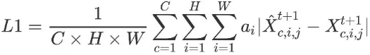
C, H, and W indicate the number of channels and the numbers of grid points in the latitude and longitude directions, respectively. c, i, and j are the indexes of the variable, latitude, and longitude coordinates, respectively. a__i indicates the weight at latitude i. As the latitude increases, the value of a__i decreases. Finally, the absolute errors of a variable and location (latitude and longitude coordinates) are summed up.

2. Fine-tuning cascaded models

After pre-training, the basic FuXi model is fine-tuned to achieve the best performance of every 6 hours from 0 to 5 days (0 to 20 time steps). This fine-tuning process applies an autoregressive regime and generates 20 time steps, which is similar to GraphCast. The fine-tuned model is called FuXi-Short.

The weights of FuXi-Short are used to initialize the FuXi-Medium model. Then the model is fine-tuned to achieve the best forecast performance for 5 days to 10 days (21-40 time steps). The output of the FuXi-Short model in the 20th time step (day 5) is the input of the FuXi-Medium model. Performing online inference of the FuXi-Short model in real time will significantly consume memory and reduce the fine-tuning speed. Therefore, data within six years (2012–2017) is calculated in advance and the output result of the FuXi-Short model is cached to the hard drive.

Finally, after Fuxi-Long applies the same process, the three models are cascaded to form a complete 15-day forecast. The cascading design helps reduce the accumulation of errors and improve the performance of long-term forecast, as shown in the figure.

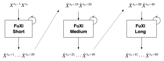
Figure 2 Cascade model architecture

Evaluation Method and Result Analysis

RMSE and ACC are calculated as follows. D indicates the test dataset, and τ indicates the forecast lead time steps. To compare the performance of the FuXi model with that of the benchmark model, (RMSE__A – RMSE__B_)/RMSE__B_ and (ACC__A – ACC__B_)/(1 – ACC__B__)_ are visualized.

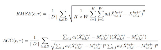
The test dataset data came from 2018. Two initialization times (00:00 UTC and 12:00 UTC) per day are selected to produce a 15-day forecast every 6 hours. To evaluate the performance of ECMWF HRES and EM models, the verification method applied by ECMWF is used in the study. In this verification method, the model analysis data (HRES-fc0 and ENS-fc0) is used as the ground truth values of the HRES and EM models, respectively.

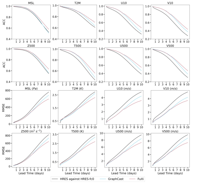
Figure 3 Comparison of globally-averaged latitude-weighted ACC and RMSE of HRES, GraphCast, and FuXi

As shown in the figure, the performance of FuXi and GraphCast is obviously better than that of ECMWF HRES. FuXi and GraphCast have similar performance within 7 days of forecast. However, after seven days, FuXi delivers better performance, with the lowest RMSE value and the highest ACC value in all variables and prediction lead time. In addition, as the lead time increases, the advantages of FuXi become more and more significant. Noticeably, FuXi also outperforms ECMWF HRES and GraphCast in variables that are not shown in the figure.

ECMWF EM, on the other hand, is used as the baseline for the 15-day forecast of normalized differences in ACC and RMSE. In the 0–9 day forecasts, FuXi outperforms ECMWF EM. The normalized ACC difference is a positive value, and the normalized RMSE difference is a negative value. However, for forecasts of more than nine days, FuXi's performance is slightly inferior to ECMWF EM, as shown in the following figure.

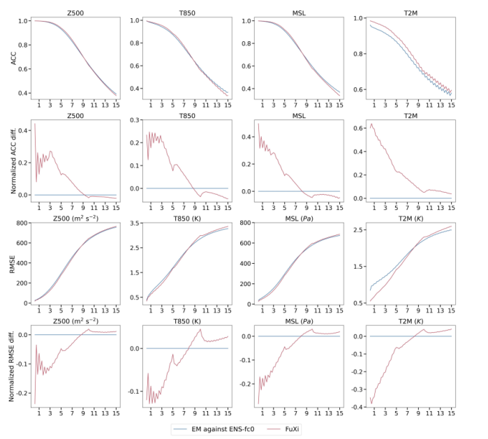
Figure 4 Comparison of the globally-averaged latitude-weighted ACC and RMSE as well as normalized ACC and RMSE difference of ECMWF EM and FuXi

Further, according to the spatial distribution visualization of the average RMSE of FuXi, the RMSE difference between ECMWF HRES and FuXi, and the RMSE difference between ECMWF EM and FuXi, the spatial error distributions of the three forecasts are similar. The highest RMSE values appear at high latitudes, while relatively small values appear at low and medium latitudes. On land, the RMSE value is higher than that on sea. The RMSE difference between ECMWF HRES and FuXi shows that FuXi outperforms ECMWF HRES at most grid points, as shown in red. In contrast, ECMWF EM performs comparable with FuXi in most areas, as shown by the predominantly white color.

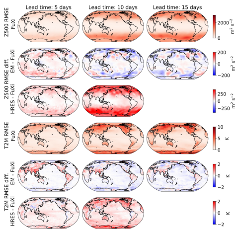
Figure 5 Spatial map of average RMSE of FuXi, the difference in RMSE between ECMWF HRES and FuXi, and the difference in RMSE between EM and FuXi

Finally, although FuXi delivers comparable performance with ECMWF EM as a cascaded model in the 15-day forecast, a limitation of current weather forecast methods based on machine learning is that they are not completely end-to-end. They still rely on analysis data generated by conventional NWP models for initial conditions. Therefore, it is also a future trend to develop a data-driven data assimilation method and use observation data to generate initial conditions for weather forecast systems based on machine learning. In this way, a real end-to-end, systematically unbiased, and computationally efficient machine learning–based weather forecast system can be constructed.

[1] Bi, K., Xie, L., Zhang, H., Chen, X., Gu, X., Tian, Q.: Pangu-Weather:A 3D High-Resolution Model for Fast and Accurate Global Weather Forecast (2022)

[2] Lam, R., Sanchez-Gonzalez, A., Willson, M., Wirnsberger, P., Fortunato,M., Pritzel, A., Ravuri, S., Ewalds, T., Alet, F., Eaton-Rosen, Z., Hu, W.,Merose, A., Hoyer, S., Holland, G., Stott, J., Vinyals, O., Mohamed, S.,

Battaglia, P.: GraphCast: Learning skillful medium-range global weather forecasting (2022)

[3] Chen L, Zhong X, Zhang F, et al. FuXi: A cascade machine learning forecasting system for 15-day global weather forecast (2023)

[4] Hersbach, H., Bell, B., Berrisford, P., Hirahara, S., Hor´anyi, A., Mu˜noz-Sabater, J., Nicolas, J., Peubey, C., Radu, R., Schepers, D., et al.: The era5 global reanalysis. Quarterly Journal of the Royal Meteorological Society146(730), 1999–2049 (2020)

[5] Liu, Z., Hu, H., Lin, Y., Yao, Z., Xie, Z., Wei, Y., Ning, J., Cao, Y., Zhang, Z., Dong, L., Wei, F., Guo, B.: Swin Transformer V2: Scaling Up Capacity and Resolution (2022)