二维圆柱绕流

本案例要求MindSpore版本 >= 2.0.0调用如下接口: mindspore.jit，mindspore.jit_class，mindspore.jacrev。

概述

圆柱绕流，是指二维圆柱低速定常绕流的流型只与Re数有关。在Re≤1时，流场中的惯性力与粘性力相比居次要地位，圆柱上下游的流线前后对称，阻力系数近似与Re成反比，此Re数范围的绕流称为斯托克斯区；随着Re的增大，圆柱上下游的流线逐渐失去对称性。这种特殊的现象反映了流体与物体表面相互作用的奇特本质，求解圆柱绕流则是流体力学中的经典问题。

由于控制方程纳维-斯托克斯方程（Navier-Stokes equation）难以得到泛化的理论解，使用数值方法对圆柱绕流场景下控制方程进行求解，从而预测流场的流动，成为计算流体力学中的样板问题。传统求解方法通常需要对流体进行精细离散化，以捕获需要建模的现象。因此，传统有限元法（finite element method，FEM）和有限差分法（finite difference method，FDM）往往成本比较大。

物理启发的神经网络方法（Physics-informed Neural Networks），以下简称PINNs，通过使用逼近控制方程的损失函数以及简单的网络构型，为快速求解复杂流体问题提供了新的方法。本案例利用神经网络数据驱动特性，结合PINNs求解圆柱绕流问题。

问题描述

纳维-斯托克斯方程（Navier-Stokes equation），简称N-S方程，是流体力学领域的经典偏微分方程，在粘性不可压缩情况下，无量纲N-S方程的形式如下：

\[\frac{\partial u}{\partial x} + \frac{\partial v}{\partial y} = 0\]

\[\frac{\partial u} {\partial t} + u \frac{\partial u}{\partial x} + v \frac{\partial u}{\partial y} = - \frac{\partial p}{\partial x} + \frac{1} {Re} (\frac{\partial^2u}{\partial x^2} + \frac{\partial^2u}{\partial y^2})\]

\[\frac{\partial v} {\partial t} + u \frac{\partial v}{\partial x} + v \frac{\partial v}{\partial y} = - \frac{\partial p}{\partial y} + \frac{1} {Re} (\frac{\partial^2v}{\partial x^2} + \frac{\partial^2v}{\partial y^2})\]

其中，Re表示雷诺数。

本案例利用PINNs方法学习位置和时间到相应流场物理量的映射，实现N-S方程的求解：

\[(x, y, t) \mapsto (u, v, p)\]

技术路径

MindFlow求解该问题的具体流程如下：

创建数据集。
构建模型。
自适应损失的多任务学习。
优化器。
NavierStokes2D。
模型训练。
模型推理及可视化

[1]:

import time

import numpy as np

import mindspore
from mindspore import context, nn, ops, Tensor, jit, set_seed, load_checkpoint, load_param_into_net
from mindspore import dtype as mstype

下述src包可以在applications/physics_driven/flow_past_cylinder/src下载。

[2]:

from mindflow.cell import MultiScaleFCCell
from mindflow.loss import MTLWeightedLossCell
from mindflow.pde import NavierStokes, sympy_to_mindspore
from mindflow.utils import load_yaml_config

from src import create_training_dataset, create_test_dataset, calculate_l2_error


set_seed(123456)
np.random.seed(123456)

[3]:

# set context for training: using graph mode for high performance training with GPU acceleration
config = load_yaml_config('cylinder_flow.yaml')
context.set_context(mode=context.GRAPH_MODE, device_target="GPU", device_id=3)
use_ascend = context.get_context(attr_key='device_target') == "Ascend"

创建数据集

本案例对已有的雷诺数为100的标准圆柱绕流进行初始条件和边界条件数据的采样。对于训练数据集，构建平面矩形的问题域以及时间维度，再对已知的初始条件，边界条件采样；基于已有的流场中的点构造测试集。

下载训练与测试数据集： physics_driven/flow_past_cylinder/dataset 。

[4]:

# create training dataset
cylinder_flow_train_dataset = create_training_dataset(config)
cylinder_dataset = cylinder_flow_train_dataset.create_dataset(batch_size=config["train_batch_size"],
                                                              shuffle=True,
                                                              prebatched_data=True,
                                                              drop_remainder=True)

# create test dataset
inputs, label = create_test_dataset(config["test_data_path"])

./flow_past_cylinder/dataset
get dataset path: ./flow_past_cylinder/dataset
check eval dataset length: (36, 100, 50, 3)

构建模型

本示例使用一个简单的全连接网络，深度为6层，激活函数是tanh函数。

[5]:

coord_min = np.array(config["geometry"]["coord_min"] + [config["geometry"]["time_min"]]).astype(np.float32)
coord_max = np.array(config["geometry"]["coord_max"] + [config["geometry"]["time_max"]]).astype(np.float32)
input_center = list(0.5 * (coord_max + coord_min))
input_scale = list(2.0 / (coord_max - coord_min))
model = MultiScaleFCCell(in_channels=config["model"]["in_channels"],
                         out_channels=config["model"]["out_channels"],
                         layers=config["model"]["layers"],
                         neurons=config["model"]["neurons"],
                         residual=config["model"]["residual"],
                         act='tanh',
                         num_scales=1,
                         input_scale=input_scale,
                         input_center=input_center)

自适应损失的多任务学习

同一时间，基于PINNs的方法需要优化多个loss，给优化过程带来的巨大的挑战。我们采用Kendall, Alex, Yarin Gal, and Roberto Cipolla. “Multi-task learning using uncertainty to weigh losses for scene geometry and semantics.” CVPR, 2018. 论文中提出的不确定性权重算法动态调整权重。

[6]:

mtl = MTLWeightedLossCell(num_losses=cylinder_flow_train_dataset.num_dataset)

优化器

[7]:

if config["load_ckpt"]:
    param_dict = load_checkpoint(config["load_ckpt_path"])
    load_param_into_net(model, param_dict)
    load_param_into_net(mtl, param_dict)

# define optimizer
params = model.trainable_params() + mtl.trainable_params()
optimizer = nn.Adam(params, config["optimizer"]["initial_lr"])

NavierStokes2D

下述NavierStokes2D将圆柱绕流问题同数据集关联起来，包含3个部分：控制方程，边界条件和初始条件。

[8]:

class NavierStokes2D(NavierStokes):
    def __init__(self, model, re=100, loss_fn=nn.MSELoss()):
        super(NavierStokes2D, self).__init__(model, re=re, loss_fn=loss_fn)
        self.ic_nodes = sympy_to_mindspore(self.ic(), self.in_vars, self.out_vars)
        self.bc_nodes = sympy_to_mindspore(self.bc(), self.in_vars, self.out_vars)

    def ic(self):
        ic_u = self.u
        ic_v = self.v
        equations = {"ic_u": ic_u, "ic_v": ic_v}
        return equations

    def bc(self):
        bc_u = self.u
        bc_v = self.v
        bc_p = self.p
        equations = {"bc_u": bc_u, "bc_v": bc_v, "bc_p": bc_p}
        return equations

    def get_loss(self, pde_data, ic_data, ic_label, bc_data, bc_label):
        pde_res = self.parse_node(self.pde_nodes, inputs=pde_data)
        pde_residual = ops.Concat(1)(pde_res)
        pde_loss = self.loss_fn(pde_residual, Tensor(np.array([0.0]).astype(np.float32), mstype.float32))

        ic_res = self.parse_node(self.ic_nodes, inputs=ic_data)
        ic_residual = ops.Concat(1)(ic_res)
        ic_loss = self.loss_fn(ic_residual, ic_label)

        bc_res = self.parse_node(self.bc_nodes, inputs=bc_data)
        bc_residual = ops.Concat(1)(bc_res)
        bc_loss = self.loss_fn(bc_residual, bc_label)

        return pde_loss + ic_loss + bc_loss

模型训练

使用MindSpore >= 2.0.0的版本，可以使用函数式编程范式训练神经网络。

[9]:

def train():
    problem = NavierStokes2D(model)

    from mindspore.amp import DynamicLossScaler, auto_mixed_precision, all_finite
    if use_ascend:
        loss_scaler = DynamicLossScaler(1024, 2, 100)
        auto_mixed_precision(model, 'O3')
    else:
        loss_scaler = None

    # the loss function receives 5 data sources: pde, ic, ic_label, bc and bc_label
    def forward_fn(pde_data, ic_data, ic_label, bc_data, bc_label):
        loss = problem.get_loss(pde_data, ic_data, ic_label, bc_data, bc_label)
        if use_ascend:
            loss = loss_scaler.scale(loss)
        return loss

    grad_fn = ops.value_and_grad(forward_fn, None, optimizer.parameters, has_aux=False)

    # using jit function to accelerate training process
    @jit
    def train_step(pde_data, ic_data, ic_label, bc_data, bc_label):
        loss, grads = grad_fn(pde_data, ic_data, ic_label, bc_data, bc_label)
        if use_ascend:
            loss = loss_scaler.unscale(loss)
            if all_finite(grads):
                grads = loss_scaler.unscale(grads)

        loss = ops.depend(loss, optimizer(grads))
        return loss


    steps = config["train_steps"]
    sink_process = mindspore.data_sink(train_step, cylinder_dataset, sink_size=1)
    model.set_train()

    for step in range(steps + 1):
        local_time_beg = time.time()
        cur_loss = sink_process()
        if step % 100 == 0:
            print(f"loss: {cur_loss.asnumpy():>7f}")
            print("step: {}, time elapsed: {}ms".format(step, (time.time() - local_time_beg)*1000))
            calculate_l2_error(model, inputs, label, config)

[10]:

time_beg = time.time()
train()
print("End-to-End total time: {} s".format(time.time() - time_beg))

momentum_x: u(x, y, t)*Derivative(u(x, y, t), x) + v(x, y, t)*Derivative(u(x, y, t), y) + Derivative(p(x, y, t), x) + Derivative(u(x, y, t), t) - 0.00999999977648258*Derivative(u(x, y, t), (x, 2)) - 0.00999999977648258*Derivative(u(x, y, t), (y, 2))
    Item numbers of current derivative formula nodes: 6
momentum_y: u(x, y, t)*Derivative(v(x, y, t), x) + v(x, y, t)*Derivative(v(x, y, t), y) + Derivative(p(x, y, t), y) + Derivative(v(x, y, t), t) - 0.00999999977648258*Derivative(v(x, y, t), (x, 2)) - 0.00999999977648258*Derivative(v(x, y, t), (y, 2))
    Item numbers of current derivative formula nodes: 6
continuty: Derivative(u(x, y, t), x) + Derivative(v(x, y, t), y)
    Item numbers of current derivative formula nodes: 2
ic_u: u(x, y, t)
    Item numbers of current derivative formula nodes: 1
ic_v: v(x, y, t)
    Item numbers of current derivative formula nodes: 1
bc_u: u(x, y, t)
    Item numbers of current derivative formula nodes: 1
bc_v: v(x, y, t)
    Item numbers of current derivative formula nodes: 1
bc_p: p(x, y, t)
    Item numbers of current derivative formula nodes: 1
loss: 0.762854
step: 0, time elapsed: 8018.740892410278ms
    predict total time: 348.56629371643066 ms
    l2_error, U:  0.929843072812499 , V:  1.0664025634627166 , P:  1.2470654215761847 , Total:  0.9487255679809018
==================================================================================================
loss: 0.099878
step: 100, time elapsed: 364.26734924316406ms
    predict total time: 26.329755783081055 ms
    l2_error, U:  0.32336308802455266 , V:  0.9999815366016505 , P:  0.7799935842779347 , Total:  0.43305926535738415
==================================================================================================
loss: 0.099729
step: 200, time elapsed: 365.6139373779297ms
    predict total time: 31.240463256835938 ms
    l2_error, U:  0.3234011910681541 , V:  1.0001619978094591 , P:  0.7813910733696886 , Total:  0.4331668769990714
==================================================================================================
loss: 0.093919
step: 300, time elapsed: 367.8765296936035ms
    predict total time: 25.576353073120117 ms
    l2_error, U:  0.30047520000238387 , V:  1.000794648538466 , P:  0.79058399174337 , Total:  0.4185132401858534
==================================================================================================
loss: 0.054179
step: 400, time elapsed: 364.1970157623291ms
    predict total time: 29.039621353149414 ms
    l2_error, U:  0.20330252312566804 , V:  0.9996817093977537 , P:  0.7340101922590306 , Total:  0.359612937152551
==================================================================================================
...
==================================================================================================
loss: 0.000437
step: 11700, time elapsed: 369.844913482666ms
    predict total time: 98.89841079711914 ms
    l2_error, U:  0.05508347849471555 , V:  0.21316098417551024 , P:  0.2859434784168006 , Total:  0.08947950657758963
==================================================================================================
loss: 0.000499
step: 11800, time elapsed: 380.2335262298584ms
    predict total time: 108.20960998535156 ms
    l2_error, U:  0.054145983320779696 , V:  0.21175303254015415 , P:  0.28978443844341173 , Total:  0.08892416803453118
==================================================================================================
loss: 0.000634
step: 11900, time elapsed: 396.8188762664795ms
    predict total time: 98.45995903015137 ms
    l2_error, U:  0.05270965792134252 , V:  0.2132374431010393 , P:  0.29610047782600435 , Total:  0.08883453152457486
==================================================================================================
loss: 0.000495
step: 12000, time elapsed: 373.43478202819824ms
    predict total time: 89.78271484375 ms
    l2_error, U:  0.05282220780283167 , V:  0.20572236320159534 , P:  0.28065431462629 , Total:  0.0864571051248727
==================================================================================================
End-to-End total time: 4497.61700296402 s

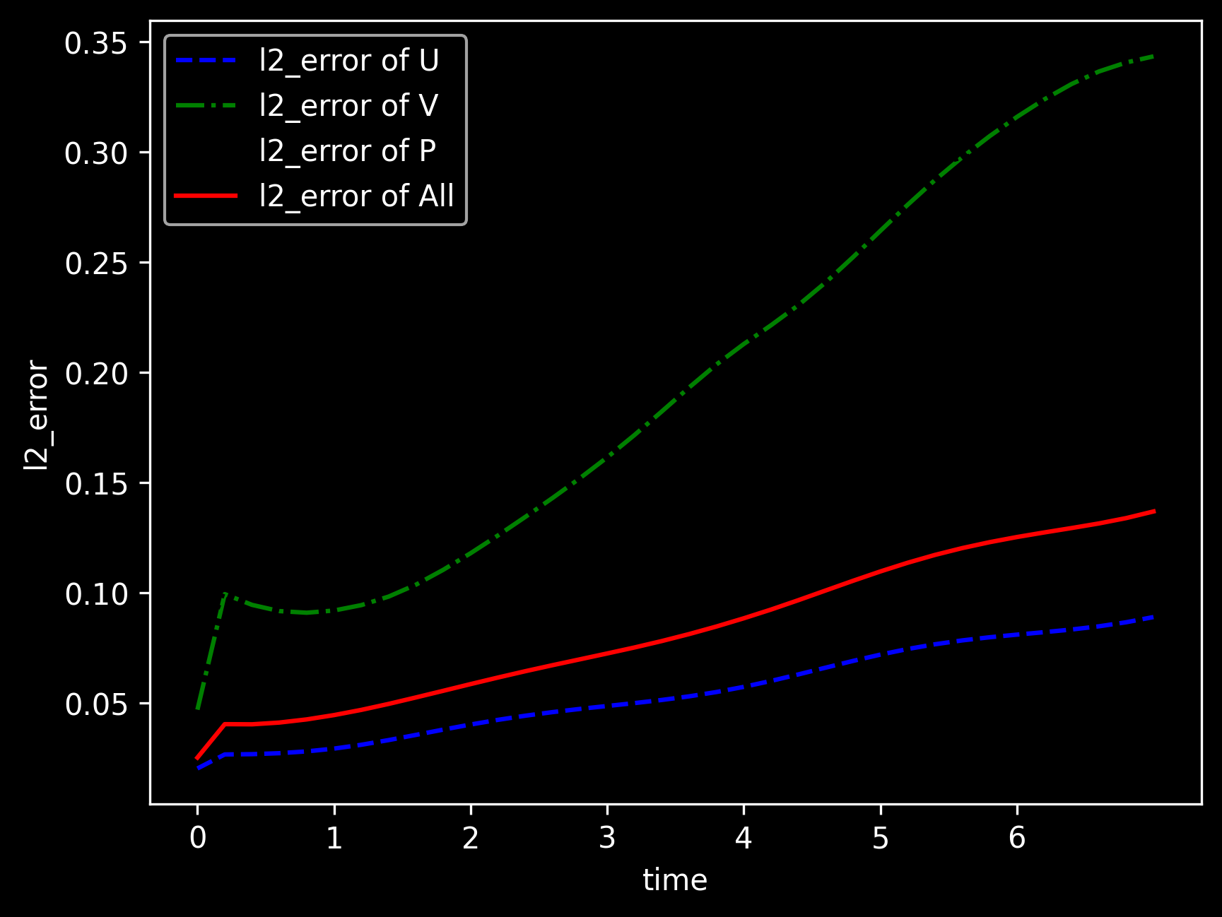
模型推理及可视化

训练后可对流场内所有数据点进行推理，并可视化相关结果。

[11]:

from src import visualization

# visualization
visualization(model=model, step=config["train_steps"], input_data=inputs, label=label)

../_images/physics_driven_navier_stokes2D_22_0.png