PhyMPGN: Physics-encoded Message Passing Graph Network for spatiotemporal PDE systems
![]()
![]()
![]()
Complex dynamical systems governed by partial differential equations (PDEs) exist in a wide variety of disciplines. Recent progresses have demonstrated grand benefits of data-driven neural-based models for predicting spatiotemporal dynamics.
Physics-encoded Message Passing Graph Network (PhyMPGN) is capable to model spatiotemporal PDE systems on irregular meshes given small training datasets. Specifically:
A physics-encoded grapph learning model with the message-passing mechanism is proposed, where the temporal marching is realized via a second-order numerical integrator (e.g. Runge-Kutta scheme)
Considering the universality of diffusion processes in physical phenomena, a learnable Laplace Block is designed, which encodes the discrete Laplace-Beltrami operator
A novel padding strategy to encode different types of BCs into the learning model is proposed.
Paper link: https://arxiv.org/abs/2410.01337
Problem Setup
Let’s consider complex physical systems, governed by spatiotemporal PDEs in the general form:
where \(\boldsymbol u(\boldsymbol x, y) \in \mathbb{R}^m\) is the vector of state variable with \(m\) components,such as velocity, temperature or pressure, defined over the spatiotemporal domain \(\{ \boldsymbol x, t \} \in \Omega \times [0, \mathcal{T}]\). Here, \(\dot{\boldsymbol u}\) denotes the derivative with respect to time and \(\boldsymbol F\) is a nonlinear operator that depends on the current state \(\boldsymbol u\) and its spatial derivatives.
We focus on a spatial domain \(\Omega\) with non-uniformly and sparsely observed nodes \(\{ \boldsymbol x_0, \dots, \boldsymbol x_{N-1} \}\) (e.g., on an unstructured mesh). Observations \(\{ \boldsymbol U(t_0), \dots, \boldsymbol U(t_{T-1}) \}\) are collected at time points \(t_0, ... \dots, t_{T- 1}\), where \(\boldsymbol U(t_i) = \{ \boldsymbol u(\boldsymbol x_0, t_i), \dots, \boldsymbol u (\boldsymbol x_{N-1}, t_i) \}\) denote the physical quantities. Considering that many physical phenomena involve diffusion processes, we assume the diffusion term in the PDE is known as a priori knowledge. Our goal is to develop a graph learning model with small training datasets capable of accurately predicting various spatiotemporal dynamics on coarse unstructured meshes, handling different types of BCs, and producing the trajectory of dynamics for an arbitrarily given IC.
This case demonstrates how PhyMPGN solves the cylinder flow problem.
The dynamical system of two-dimensional cylinder flow is governed by Navier-Stokes equation
Where the fluid density \(\rho\) is 1,the fluid viscosity \(\mu\) is \(5\times10^{-3}\),and the external force \(f\) is 0。The cylinder flow system has an inlet on the left boundary, an outlet on the right boundary, a no-slip boundary condition on the cylinder surface, and symmetric boundary conditions on the top and bottom boundaries. This case study focuses on generalizing the inflow velocity \(U_m\) while keeping the fluid density \(\rho\), cylinder diameter \(D=2\), and fluid viscosity \(\mu\) constant. Since the Reynolds number is defined as \(Re=\rho U_m D/ \mu\), generalizing the inflow velocity \(U_m\) inherently means generalizing different Reynolds numbers.
Model Architecture
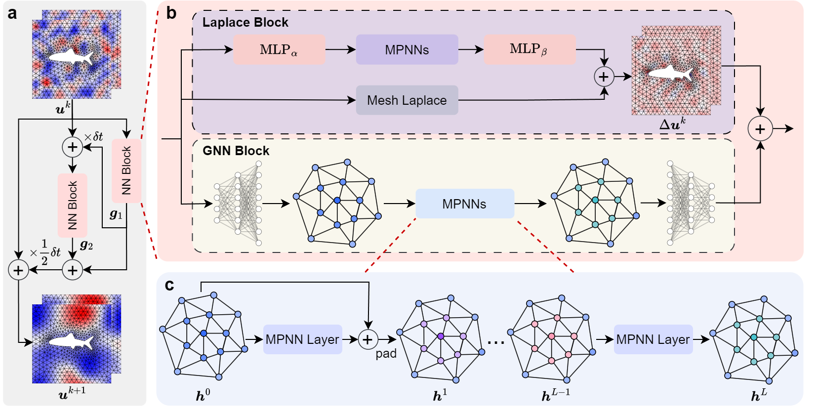
For Equation (1), a second-order Runge-Kutta (RK2) scheme can be used for discretization:
where \(\boldsymbol u^k\) is the state variable at time \(t^k\),and \(\delta t\) denotes the time interval between \(t^k\) and \(t^{k+1}\). According to the Equation (2), we develop a GNN to learn the nonlinear operator \(\boldsymbol F\).
As shown in Figure, the NN block aims to learn the nonlinear operator \(\boldsymbol F\) and consists of two parts: a GNN block followed the Encode-Process-Decode module and a learnable Laplace block. Due to the universality of diffusion processes in physical phenomena, we design the learnable Laplace block, which encodes the discrete Laplace-Beltrami operator, to learn the increment caused by the diffusion term in the PDE, while the GNN block is responsible to learn the increment induced by other unknown mechanisms or sources.
Preparation
Make sure the required dependency libraries (such as MindSpore) have been installed
Ensure the cylinder flow dataset has been downloaded
Verify that the data and model weight storage paths have been properly configured in the yamls/train.yaml configuration file
Code Execution Steps
The code execution flow consists of the following steps:
Read configuration file
Build dataset
Construct model
Model training
Model inference
Reading Configuration File
[1]:
from mindflow.utils import log_config, load_yaml_config, print_log
from easydict import EasyDict
import os.path as osp
from pathlib import Path


def load_config(config_file_path, train):
    config = load_yaml_config(config_file_path)
    config['train'] = train
    config = EasyDict(config)
    log_dir = './logs'
    if train:
        log_file = f'phympgn-{config.experiment_name}'
    else:
        log_file = f'phympgn-{config.experiment_name}-te'
    if not osp.exists(osp.join(log_dir, f'{log_file}.log')):
        Path(osp.join(log_dir, f'{log_file}.log')).touch()
    log_config(log_dir, log_file)
    print_log(config)
    return config
[ ]:
config_file_path = 'yamls/train.yaml'
config = load_config(config_file_path=config_file_path, train=True)
[ ]:
import mindspore as ms

ms.set_device(device_target='Ascend', device_id=7)
Building Dataset
[ ]:
from src import PDECFDataset, get_data_loader


print_log('Train...')
print_log('Loading training data...')
tr_dataset = PDECFDataset(
    root=config.path.data_root_dir,
    raw_files=config.path.tr_raw_data,
    dataset_start=config.data.dataset_start,
    dataset_used=config.data.dataset_used,
    time_start=config.data.time_start,
    time_used=config.data.time_used,
    window_size=config.data.tr_window_size,
    training=True
)
tr_loader = get_data_loader(
    dataset=tr_dataset,
    batch_size=config.optim.batch_size
)

print_log('Loading validation data...')
val_dataset = PDECFDataset(
    root=config.path.data_root_dir,
    raw_files=config.path.val_raw_data,
    dataset_start=config.data.dataset_start,
    dataset_used=config.data.dataset_used,
    time_start=config.data.time_start,
    time_used=config.data.time_used,
    window_size=config.data.val_window_size
)
val_loader = get_data_loader(
    dataset=val_dataset,
    batch_size=config.optim.batch_size
)
Constructing Model
[ ]:
from src import PhyMPGN

print_log('Building model...')
model = PhyMPGN(
    encoder_config=config.network.encoder_config,
    mpnn_block_config=config.network.mpnn_block_config,
    decoder_config=config.network.decoder_config,
    laplace_block_config=config.network.laplace_block_config,
    integral=config.network.integral
)
print_log(f'Number of parameters: {model.num_params}')
Model training
[ ]:
from mindflow import get_multi_step_lr
from mindspore import nn
import numpy as np

from src import Trainer, TwoStepLoss


lr_scheduler = get_multi_step_lr(
    lr_init=config.optim.lr,
    milestones=list(np.arange(0, config.optim.start_epoch+config.optim.epochs,
                              step=config.optim.steplr_size)[1:]),
    gamma=config.optim.steplr_gamma,
    steps_per_epoch=len(tr_loader),
    last_epoch=config.optim.start_epoch+config.optim.epochs-1
)
optimizer = nn.AdamWeightDecay(model.trainable_params(), learning_rate=lr_scheduler,
                               eps=1.0e-8, weight_decay=1.0e-2)
trainer = Trainer(
    model=model, optimizer=optimizer, scheduler=lr_scheduler, config=config,
    loss_func=TwoStepLoss()
)
trainer.train(tr_loader, val_loader)
[Epoch 1/1600] Batch Time: 2.907 (3.011) Data Time: 0.021 (0.035) Graph Time: 0.004 (0.004) Grad Time: 2.863 (2.873) Optim Time: 0.006 (0.022)
[Epoch 1/1600] Batch Time: 1.766 (1.564) Data Time: 0.022 (0.044) Graph Time: 0.003 (0.004)
[Epoch 1/1600] tr_loss: 1.36e-02 val_loss: 1.29e-02 [MIN]
[Epoch 2/1600] Batch Time: 3.578 (3.181) Data Time: 0.024 (0.038) Graph Time: 0.004 (0.004) Grad Time: 3.531 (3.081) Optim Time: 0.004 (0.013)
[Epoch 2/1600] Batch Time: 1.727 (1.664) Data Time: 0.023 (0.042) Graph Time: 0.003 (0.004)
[Epoch 2/1600] tr_loss: 1.15e-02 val_loss: 9.55e-03 [MIN]
…
Model Inference
[ ]:
config_file_path = 'yamls/train.yaml'
config = load_config(config_file_path=config_file_path, train=False)
[ ]:
import mindspore as ms

ms.set_device(device_target='Ascend', device_id=7)
[ ]:
from src import PDECFDataset, get_data_loader, Trainer, PhyMPGN
from mindspore import nn


# test datasets
te_dataset = PDECFDataset(
    root=config.path.data_root_dir,
    raw_files=config.path.te_raw_data,
    dataset_start=config.data.te_dataset_start,
    dataset_used=config.data.te_dataset_used,
    time_start=config.data.time_start,
    time_used=config.data.time_used,
    window_size=config.data.te_window_size,
    training=False
)
te_loader = get_data_loader(
    dataset=te_dataset,
    batch_size=1,
    shuffle=False,
)
print_log('Building model...')
model = PhyMPGN(
    encoder_config=config.network.encoder_config,
    mpnn_block_config=config.network.mpnn_block_config,
    decoder_config=config.network.decoder_config,
    laplace_block_config=config.network.laplace_block_config,
    integral=config.network.integral
)
print_log(f'Number of parameters: {model.num_params}')
trainer = Trainer(
    model=model, optimizer=None, scheduler=None, config=config,
    loss_func=nn.MSELoss()
)
print_log('Test...')
trainer.test(te_loader)
.[TEST 0/9] MSE at 2000t: 5.06e-04, armse: 0.058, time: 185.3432s
[TEST 1/9] MSE at 2000t: 4.83e-04, armse: 0.040, time: 186.3979s
[TEST 2/9] MSE at 2000t: 1.95e-03, armse: 0.062, time: 177.0030s
…
[TEST 8/9] MSE at 2000t: 1.42e-01, armse: 0.188, time: 163.1219s
[TEST 9] Mean Loss: 4.88e-02, Mean armse: 0.137, corre: 0.978, time: 173.3827s